Differential equations on a computer: Euler, Runge-Kutta and stiff problems
Euler's method and its error, Heun and fourth-order Runge-Kutta, adaptive step, stability and stiff problems, implicit methods in SPICE and symplectic methods.
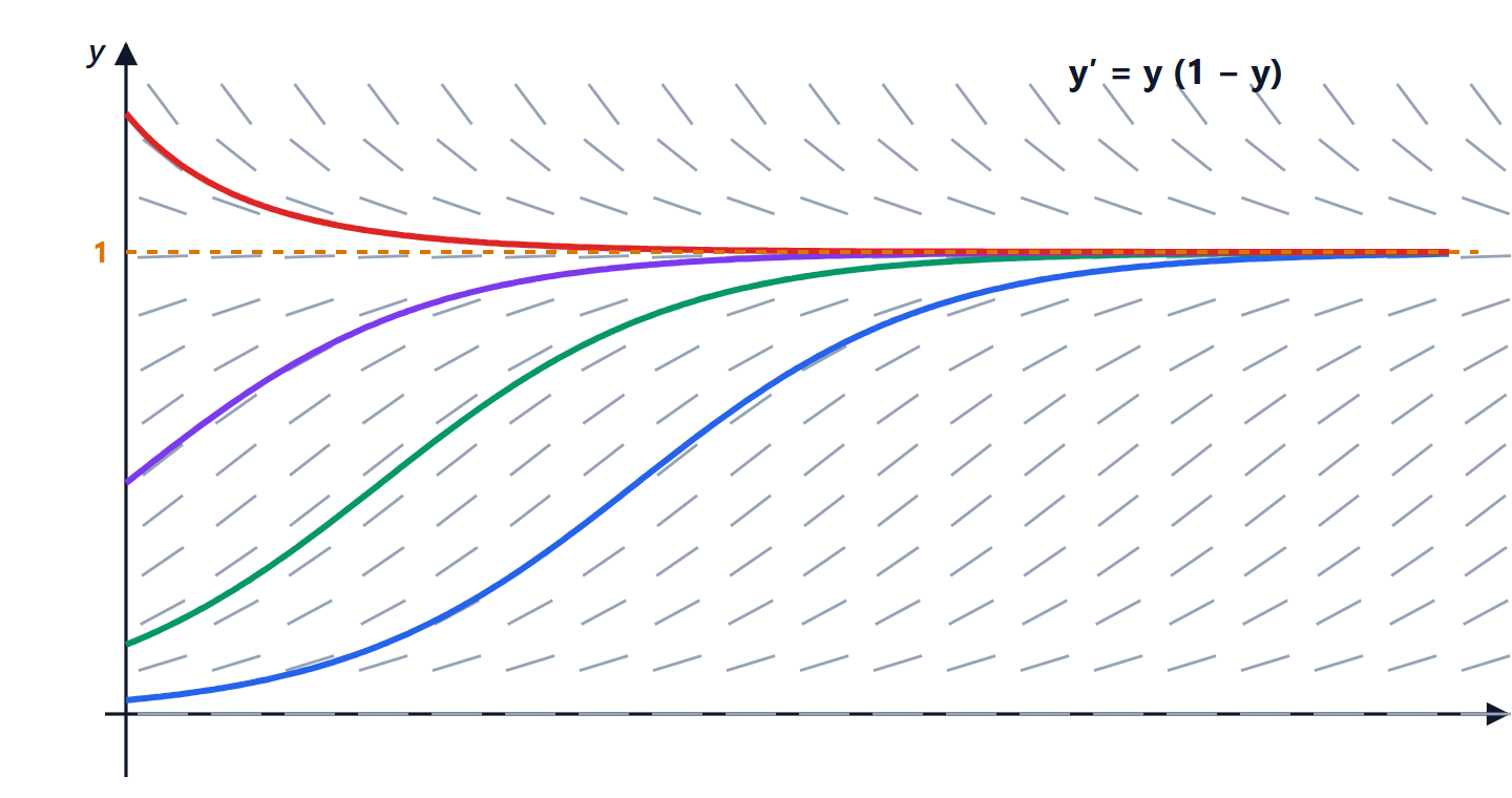
The differential equations you can solve with pen and paper are few: linear ones with constant coefficients, separable ones. A circuit with a diode, a pendulum with large swings, a motor with nonlinear friction, the orbit of a satellite around the oblate Earth all need numerical methods. The idea is simple: start from the initial condition and advance in small time steps, following the direction field. In this lesson we cover Euler’s and the Runge-Kutta methods, order of accuracy and the problem of stability.
The problem

where  can also be a vector: every higher-order equation can be rewritten as a first-order system. The pendulum
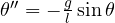 becomes
 ,
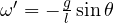 . Choose the times
 , with
 the step, and compute approximations
 .
The explicit Euler method
Follow the tangent for one step:

It is the definition of the derivative read backwards. Each step makes a local error proportional to  (the neglected Taylor term); after
 steps the global error is proportional to . Euler is a first-order method: halving the step halves the error.
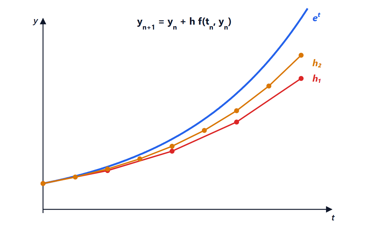
 ,
 , the exact solution is
 (blue). Euler with step
 (red) and
 (orange) stays below the true curve, because the tangent of a convex function lies below it; halving the step roughly halves the error.
Example. With Euler gives  , that is
 . To reach
 : with
 ,
 instead of
 (4.6% error); with
 ,
 (0.5% error). It is the definition of
 as the limit of
 .
Runge-Kutta methods
To get more accuracy without shrinking the step too much, evaluate the slope at several points within the step and take a weighted average. Heun’s method (second-order Runge-Kutta) takes a trial Euler step, computes the slope at the end point and uses the average of the two slopes:

The most used method is fourth-order Runge-Kutta (RK4):


Four evaluations of  per step, global error proportional to
 : halving the step cuts the error by sixteen. For with up to , RK4 gives
 against
 : an error of 2 millionths, against Euler’s 4.6% with the same step. The weights
 have the same structure as Simpson’s rule: for depending only on
 , RK4 is Simpson.
Adaptive step. Modern solvers (MATLAB’s ode45, SciPy’s solve_ivp) compute two estimates of different order at each step, use their difference as an error estimate and adjust the step: large where the solution is quiet, small where it changes quickly.
Stability and stiff problems
Apply Euler to  with
 , whose solution
 decays. Euler gives
 . If
 , that is if

the computed values grow and oscillate in sign, while the true solution goes to zero. The method is unstable. It is not a matter of accuracy: even when the solution is almost zero after a while and does not need to be followed in detail, the step must stay small.
A problem is stiff when it contains very different time constants. A circuit with one time constant of 1 ns and another of 1 ms, simulated for a few milliseconds, would force an explicit method to take steps below 2 ns throughout: millions of steps, even after the fast transient has died away.
The answer is implicit methods, such as implicit Euler:

where the slope is evaluated at the end point. For it gives 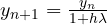 , which decays for any step. The price is that at each step an equation must be solved (or a nonlinear system, with Newton). SPICE uses exactly implicit methods, the implicit trapezoidal rule and Gear’s formulas, because electronic circuits are almost always stiff. When you change the integration method from “trap” to “gear” in a simulation’s options, you are choosing between two implicit methods with different stability properties.
Conservation of energy
For frictionless oscillating systems, such as an ideal LC circuit or an orbit, explicit Euler makes the energy grow at every turn and the trajectory spirals outwards; implicit Euler makes it shrink. There are methods, called symplectic (such as the Verlet method, used in molecular dynamics simulations and in video game physics engines), that conserve energy for very long times even with large steps.