Compensators: lead and lag networks
From specifications to the shape of the loop function, the lead network and maximum phase lead with proof, a complete design with verification, the lag network and lead-lag.
Frequency-domain design consists of giving the loop function  the right shape: high gain at low frequency for steady-state errors, a suitable crossover frequency for speed, enough phase margin for damping. The tools are compensators: the lead network adds phase near crossover, the lag network raises the low-frequency gain without touching the margin. In this lesson we derive them and complete the example from the lesson on the Nyquist criterion.
From specifications to the shape of L
Time-domain specifications are translated into frequency with approximate but widely used rules:
- phase margin
 → damping
 , hence overshoot;
- crossover frequency
 → speed: the rise time is about
 and the closed-loop bandwidth is of the same order as ;
- low-frequency gain → steady-state error (lesson on errors).
The Bode magnitude plot should cross 0 dB with a slope of about −20 dB/decade: steeper slopes at crossover mean a phase close to −180° and small margins.
The lead network

has a zero at  and a pole further left, at
 . Between the two frequencies the magnitude rises by
 dB and the phase is positive: it is a limited derivative action, which does not amplify noise without bound.
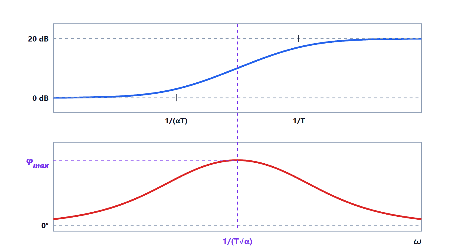
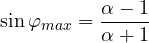
Theorem. The phase lead is largest at the frequency  , the geometric mean of zero and pole, and equals
There the magnitude is  , that is
 dB.
Proof. The phase is  . Setting
 and using the tangent of a difference:

The maximum is where the derivative with respect to  vanishes:
 , that is
 . There
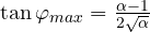 , and from the right triangle with legs
 and
 the hypotenuse is
 : so
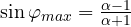 . The magnitude at is
 . ∎
 | 4 | 6 | 10 | 20 |
|---|---|---|---|---|
 | 36.9° | 45.6° | 54.9° | 64.8° |
Beyond  the phase gain grows little and the noise a lot: for larger leads two networks in cascade are used.
A complete design
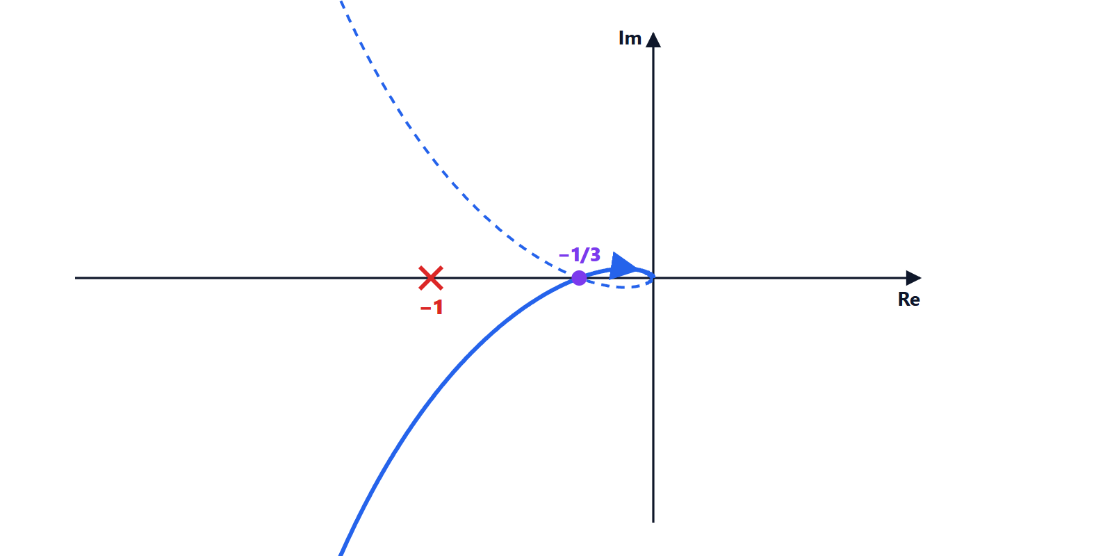
Plant and gain from the lesson on the Nyquist criterion:  , with a phase margin of 25°, too little. Goal: at least 45 to 50°.
- Choosing α. About 25 to 30° of lead is needed, plus a margin for the fact that the network moves crossover to the right, where the plant phase is worse. Try
 (
 ).
- Placement. It is best to put the phase maximum right at the new crossover. There the network adds
 dB, so the new is where the plant alone is at
 dB, that is
 : this happens at
 rad/s.
- Computing T.
 gives
 s, and the network is
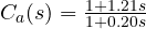 .
- Check. With the network the phase margin becomes about 50° and crossover moves from 1.23 to 2.02 rad/s: a better damped response (in simulation the overshoot drops from about 49% to 17%) and a faster one too.
With  one would get about 46°, with
 about 54°: the final choice is made by simulating and also checking the effect on noise.
The lag network

is the opposite: it attenuates high frequencies times, leaving low ones unchanged. Used together with an -fold increase in gain, it has the effect of multiplying the low-frequency gain by α (and dividing the steady-state error by α) without changing the behaviour near crossover. Its phase lag must be kept away from : the zero  is placed at least a decade below crossover.
Lead and lag networks together form a lead-lag compensator, the frequency-domain equivalent of a PID: the lag part does the work of the integral, the lead part that of the derivative.