Converter control: averaged model, voltage and current loops
The averaged model, the buck transfer function proved, voltage-mode control and type III compensator, peak current-mode control, the right-half-plane zero of the boost, digital control.
A converter must keep its output constant while the input voltage and the load change: a processor can go from a few milliamperes to tens of amperes in a microsecond. A feedback loop is needed, and to design it a model of the converter is needed, which however is a switching circuit: non-linear and time-varying. The trick is to look at its average over a switching period. In this lesson we look at the averaged model, the transfer function of the buck with proof, voltage-mode and current-mode control, the right-half-plane zero of the boost and the loop design rules.
The averaged model
If the switching frequency is much higher than the dynamics of the inductor and capacitor, the ripple is small and what matters is the mean value of the quantities over each period. In a buck the node between switch and diode equals  for a fraction
 of the period and zero for the rest: its mean value is
 . The “averaged” buck is therefore a voltage source followed by the LC filter and the load: a linear circuit, in which the duty cycle is a continuous input just like a voltage.
The transfer function of the buck
Theorem. For the buck in continuous conduction, with inductance  , capacitance
 and resistive load
 , the transfer function from small variations of the duty cycle to those of the output is

Proof. In the averaged model the voltage at the filter input is . The filter is a series inductor followed by the parallel combination of and , with impedance  ; the divider gives

With constant, a small variation  of the duty cycle produces at the filter input the variation
 , and the filter transmits it to the output with the same function. ∎
It is a second-order system with two complex poles at the frequency  and quality factor
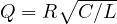 : at light load (large ) the resonance is very pronounced, and the phase drops by 180° in little more than an octave. Example. With
 µH and
 µF,
 kHz.
The voltage-mode control loop
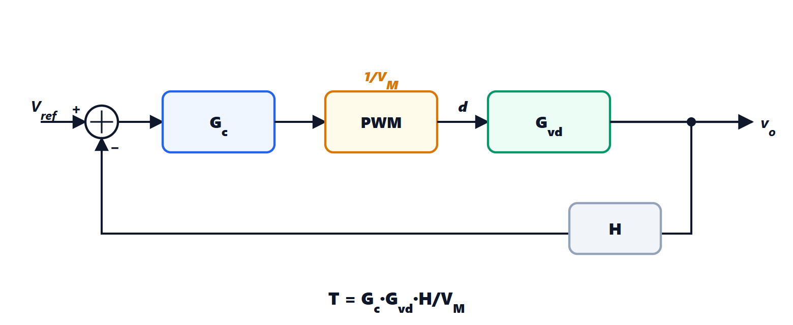
The duty cycle is produced by a PWM modulator that compares the control voltage with a ramp of amplitude  :
 . The loop gain is
 . The design follows the rules of the Automatic Control lesson on margins:
- the crossover frequency is chosen between a tenth and a fifth of the switching frequency, because the averaged model holds only at frequencies much lower than switching: with 500 kHz, around 50 kHz;
- the phase margin must be 45-60°;
- an integrator in the compensator removes the steady-state error (lesson on steady-state errors).
Since the LC filter poles remove 180° of phase before crossover, the compensator must give a lot back: the type III compensator is used, with two zeros near  and two poles at high frequencies, built with an op-amp and a few resistors and capacitors (lesson on compensators).
Current-mode control
A very widespread alternative is peak current-mode control: an inner loop turns the switch off when the inductor current reaches the value requested by the outer voltage loop. For the outer loop the inductor becomes a kind of controlled current source, and the system behaves roughly as a first-order one (the capacitor with the load): a single pole, easier to compensate. Current-mode control also naturally limits the maximum current, protecting the converter from short circuits, and shares current well among several phases in parallel. With duty cycles above 0.5 it becomes unstable at half the switching frequency (subharmonic oscillation), which is corrected by adding a compensation ramp.
The boost zero
In the boost and the buck-boost a counter-intuitive phenomenon appears: if the duty cycle is increased to raise the output, in the first instant the output falls, because the switch stays closed longer and the inductor delivers energy to the output for less time; only later, once the inductor current has grown, does the output rise. Mathematically it is a right-half-plane zero, at  , which adds phase lag like a pure delay (Process Control lesson on processes with dead time) and limits the achievable bandwidth: crossover must be kept at a fraction of the zero frequency, which drops at heavy load and high duty cycle.
Digital control
More and more converters are controlled by a microcontroller or a dedicated DSP, which samples voltages and currents and computes the duty cycle every period (Process Control lesson on digital control). Digital control makes it possible to change parameters according to conditions, to communicate with the system, and to handle start-up and protection flexibly. Computation delay and PWM resolution, a few nanoseconds, are its main limits.