Inverters: sinusoidal PWM, three-phase inverters and grid connection
The H-bridge and square wave, sinusoidal PWM with the fundamental amplitude proved, harmonics and unipolar modulation, three-phase inverter and space-vector modulation, dead time, grid inverters and MPPT.
The inverter does the opposite of the rectifier: from a DC voltage it produces an AC voltage of adjustable frequency and amplitude. It is the heart of electric cars, grid-connected photovoltaic plants, uninterruptible power supplies and every variable-speed motor, from air-conditioner compressors to trains. In this lesson we look at the H-bridge, sinusoidal pulse-width modulation with the proof of the amplitude of the fundamental, the harmonic spectrum, the three-phase inverter and the gain of space-vector modulation, dead time and grid-connected inverters.
The H-bridge
A single-phase inverter is an H-bridge: four switches, two per leg, with the load between the midpoints of the two legs. Closing one diagonal pair or the other, the load sees  or
 . Alternating the pairs at 50 Hz gives a square wave: simple, but full of harmonics (third at 33 %, fifth at 20 %…) and with a fixed fundamental amplitude,
 . To get a clean, adjustable sine wave one switches much faster.
Sinusoidal PWM
A sinusoidal reference at the desired frequency is compared with a much faster triangular carrier, of a few kilohertz or tens of kilohertz: when the reference exceeds the carrier the leg goes to , otherwise to . The ratio of the amplitudes is the modulation index  , that of the frequencies the index
 .
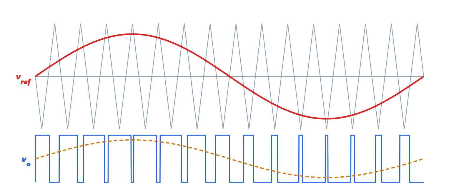
Theorem. With a carrier much faster than the reference, the mean value of the output over each switching period is

i.e. the amplitude of the fundamental is  , proportional to the modulation index, as long as
 .
Proof. In a switching period, short enough for the reference to be roughly constant and equal to  (normalised to the carrier amplitude, which goes from
 to
 ), the leg is at for the fraction of the period in which the triangle is below
 . Since the triangle sweeps linearly between and , this fraction is
 . The mean value is
 . ∎
The instantaneous voltage is always  , but the load, almost always inductive like a motor or a filter, responds to the mean value: the current is almost sinusoidal. The harmonics do not vanish, they move around the carrier frequency and its multiples, where inductance attenuates them easily. A higher carrier frequency gives cleaner currents and acoustic noise beyond audibility, but more switching losses (lesson on devices). With unipolar modulation, in which the two legs are modulated with opposite references, the output has three levels (, 0, ) and the first harmonics move to twice the switching frequency.
For  the inverter enters overmodulation: some pulses disappear, the fundamental grows less than proportionally and low harmonics reappear.
The three-phase inverter
The three-phase inverter has three legs, one per phase, and the load (a motor) connected in star without neutral. Each leg is modulated with a reference shifted by 120°. What matters to the motor are only the line-to-line voltages, differences between two phases: any component equal in the three phases (common-mode) cancels. This is exploited by adding a third harmonic to the references, or with space-vector modulation (SVPWM), which directly chooses the combinations of switch states: the maximum line-to-line voltage obtainable in the linear range grows by 15 %, a factor  , for the same DC voltage. It is the standard technique of drives (lesson on motors).
Dead time
Between turning off one switch and turning on the other of the same leg a dead time of a few hundred nanoseconds is left, to avoid short-circuiting the supply (lesson on devices). During the dead time the leg voltage is set by the direction of the current, which flows in the diode of one of the two switches: this produces a voltage error that depends on the sign of the current and distorts the waveform especially at low motor speeds. Modern controls measure it and compensate for it.
Grid-connected inverters
A photovoltaic inverter, a storage system or a car’s bidirectional charger does not impose a voltage: it connects to a grid that already has one. It therefore controls the injected current, synchronising with the grid voltage through a phase-locked loop (Electrical Communications lesson on the PLL), and regulates active and reactive power. In photovoltaics a first stage tracks the panels’ maximum power point (MPPT), continuously varying the operating point to extract the maximum power available with the current sunlight. Standards require the inverter to disconnect if the grid fails (so as not to feed a line that technicians believe dead) and, more and more often, to support the grid during voltage dips instead of tripping. Multilevel inverters, with several intermediate voltages, reduce harmonics and stresses in medium-voltage applications.





