Solved root locus exercises, with the loci drawn
Nine exercises with solutions: gain for a damping, asymptotes and breakaway, circular locus, departure angles, stabilising an unstable process, stabilising zero, locus with respect to a parameter, design for overshoot.
Root locus exercises of the kind set in Control Systems courses, in three levels: basic, with second-order systems and gain computation; intermediate, with asymptotes, breakaway points, departure angles and imaginary-axis crossings; exam, with unstable processes, compensation with a zero, locus with respect to a parameter and design to a specification. The result is given straight away; the full solution, with the locus drawn, opens with a click. The proved rules and the MATLAB and Python code are in the in-depth study linked at the top.
Basic level
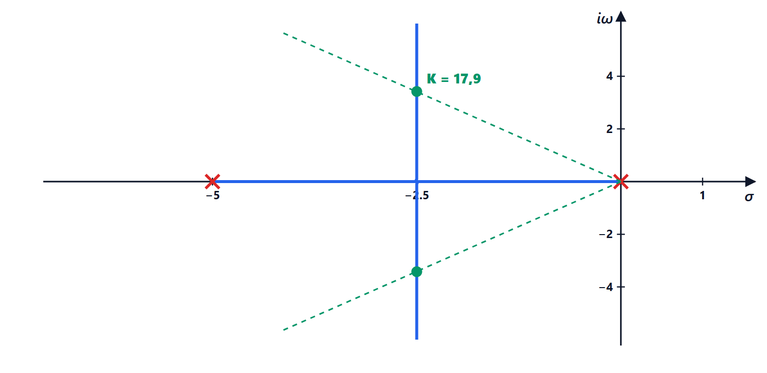
Exercise 1. The simplest locus
Sketch the locus of  and find the gain for which the closed-loop poles have damping
 .
Result: branches on the real axis between 0 and  , breakaway at
 for
 , then the vertical line
 ;
 .
Solution
Characteristic equation:  . Real axis: the stretch between 0 and (to the right of each of its points there is one pole). Two asymptotes at
 from the centroid
 .
Breakaway:  ,
 , with . For
 the poles are
 : the real part stays at (the sum of the poles is constant, rule 7).
Damping: comparing with  ,
 and
 . For : , poles
 . Increasing the gain makes the response more oscillatory but not faster to settle: the settling time
 s does not change.

Exercise 2. A gain for an overshoot
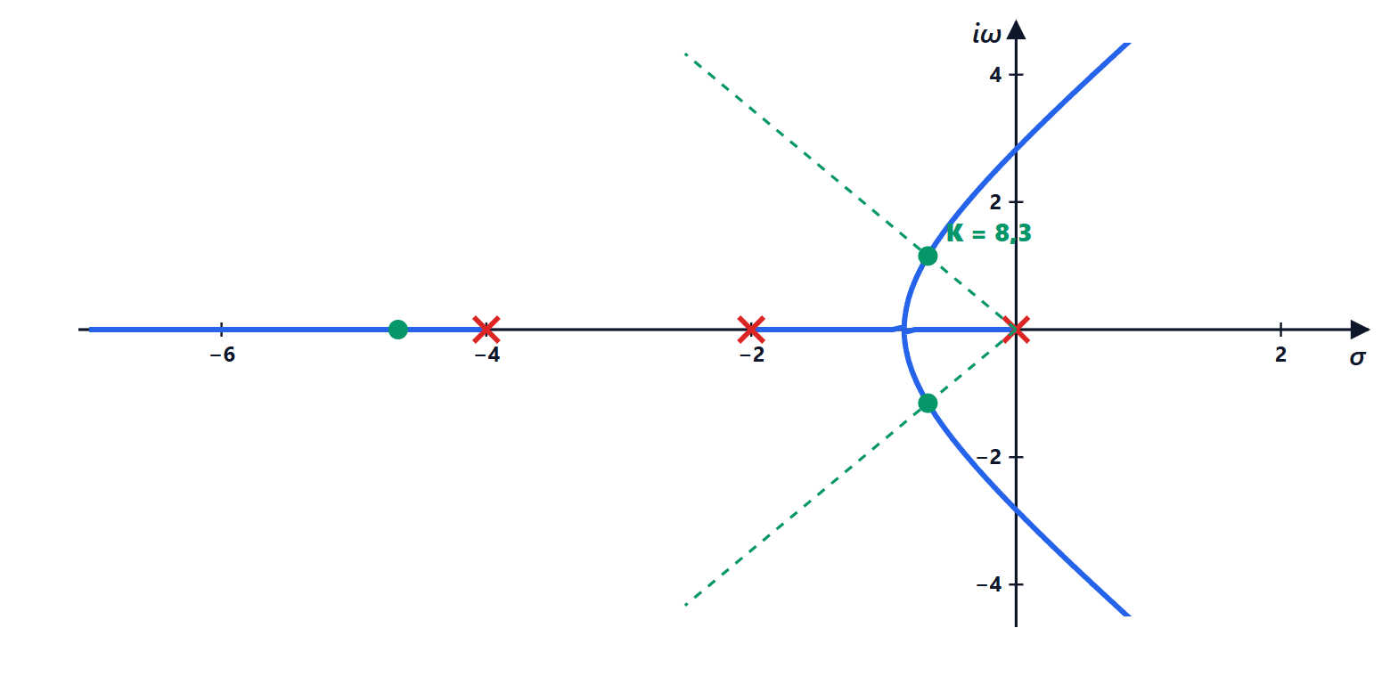
For 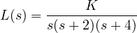 find the gain that gives the dominant poles a damping of 0.5, the position of the third pole and the critical gain.
Result:  ; dominant poles
 , third pole
 ;
 .
Solution
The dominant poles lie on the line  (damping 0.5, angle 60° from the negative half-axis). By rule 7, the sum of the three poles is always
 : if the dominant ones are
 , the third is
 .
Requiring  , the coefficient of
 gives
 , i.e.
 ,
 . Then the dominant poles are , the third , and
 .
Critical gain (Routh, or  ):
 ,
 ,
 . The gain margin with is
 .
The third pole is seven times further from the axis than the dominant ones: its influence is small, and the actual overshoot (15.5 %) is close to that of the second-order system (16.3 %).
Intermediate level
Exercise 3. Four poles: asymptotes, breakaway, stability
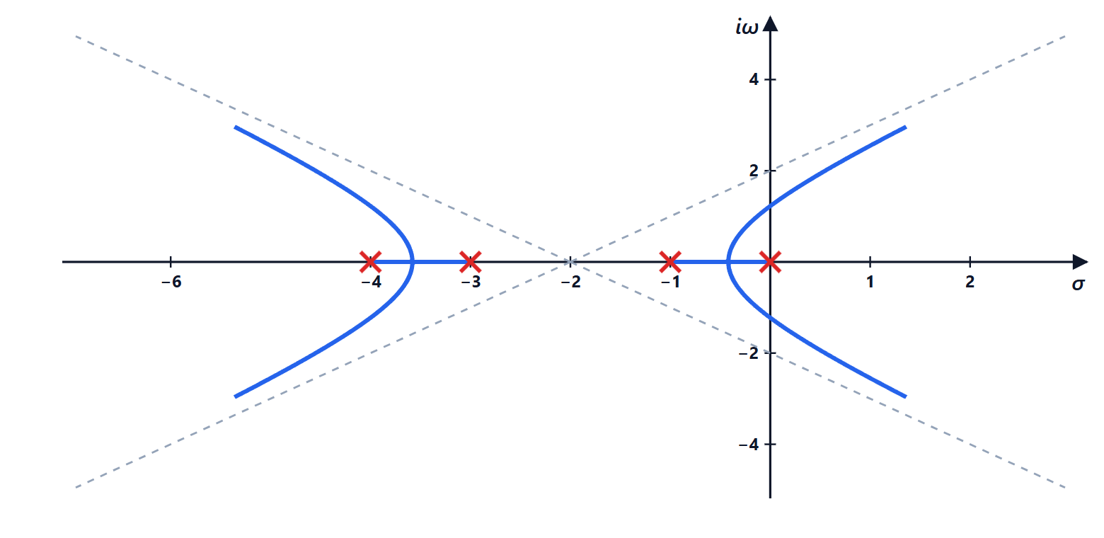
For  find the asymptotes, the breakaway points and the critical gain.
Result: centroid , angles  and
 ; breakaway at
 and
 (both with
 );
 with
 .
Solution
Real axis: stretches  and
 . Asymptotes:
 , centroid
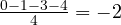 , angles
 .
Breakaway:  ,
 : roots , , . The point is not on the locus (between and
 there are two poles to the right, an even number). At the other two
 : the same
 by symmetry (the poles are symmetric about ).
Routh on  : second row
 ; third
 and ; fourth
 , positive for
 . Auxiliary equation
 : .
Exercise 4. The circular locus and maximum damping
For 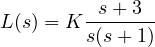 find the breakaway points and the gain that gives maximum damping of the complex poles.
Result: breakaway at  and
 ; maximum damping
 for , with poles
 .
Solution
Breakaway (in-depth study):  ,
 .
The complex part of the locus is the circle centred at with radius  . The damping of a pole is the cosine of the angle between the line to the origin and the negative half-axis: it is maximum where the line from the origin is tangent to the circle. There
 ,
 , and the distance from the origin is
 .
The pole is  . From the equation
 , the real part is
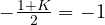 , so . Check:
 has roots .
Exercise 5. Departure angle and crossing
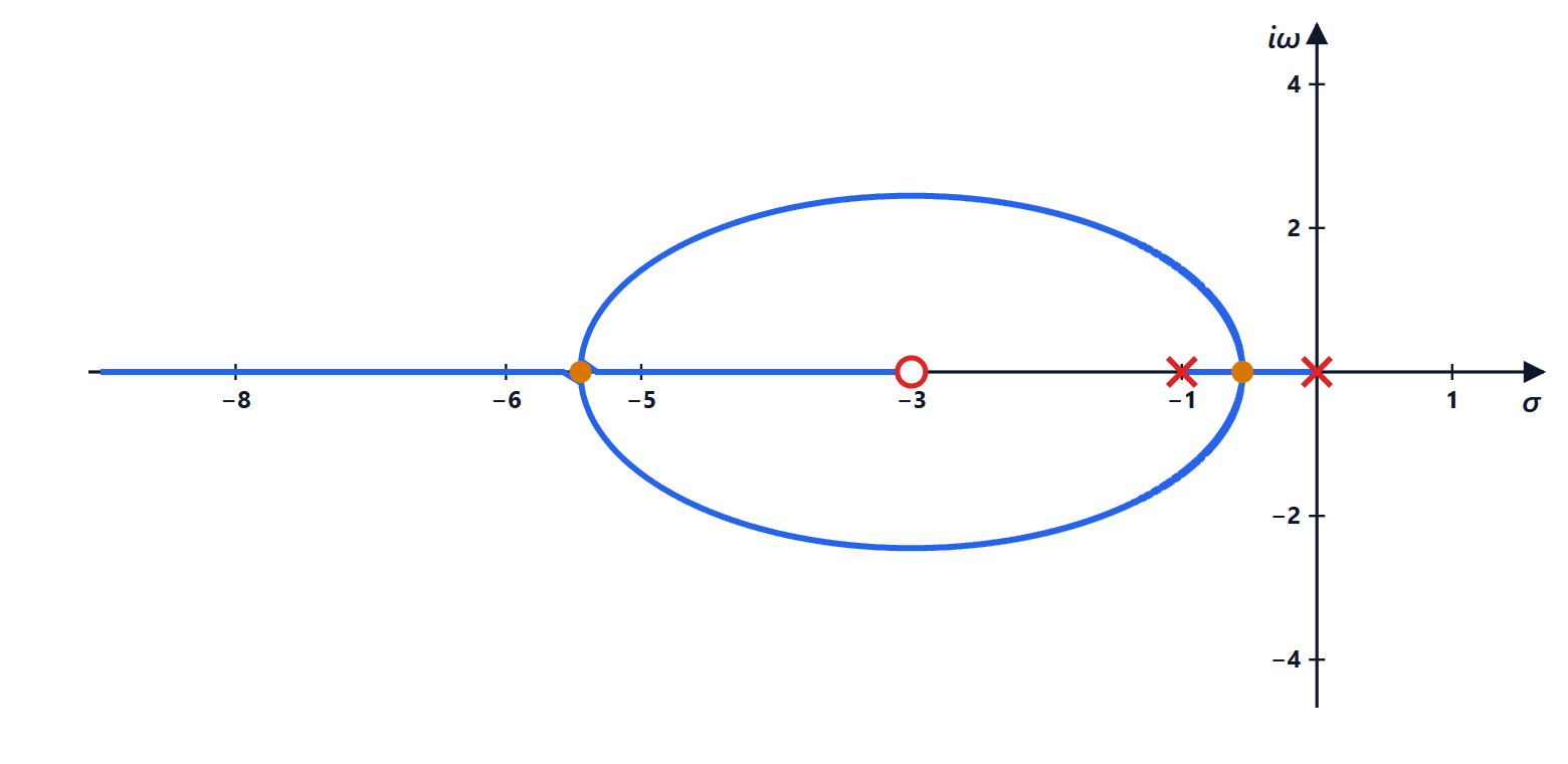
For  compute the departure angle from the pole
 , the asymptotes and the critical gain.
Result:  ; centroid
 , angles
 ,
 ;
 with
 .
Solution
Departure (rule 6):  .
Asymptotes:  .
Characteristic equation  . Routh:
 , i.e.
 . For
 :
 ,
 .
Check with rule 7: for the poles are  and the third must be
 (sum ): indeed
 . ✓
Exam level
Exercise 6. Stabilising an unstable process
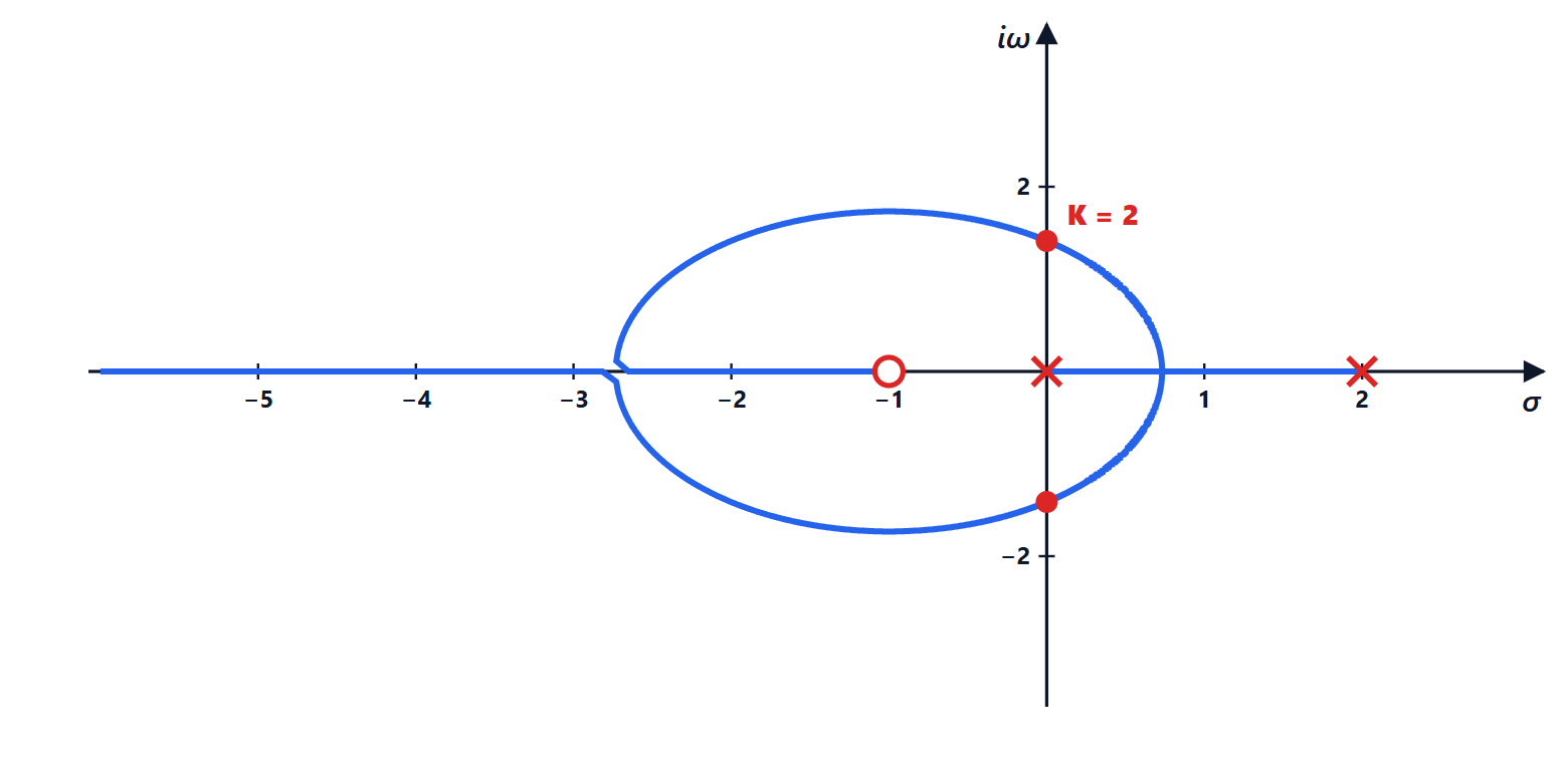
The process 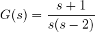 is controlled with a gain in unity feedback. For which is the closed loop stable? For which are the poles real and coincident?
Result: stable for  ; coincident poles for
 , at
 (and for
 , at
 , unstable).
Solution
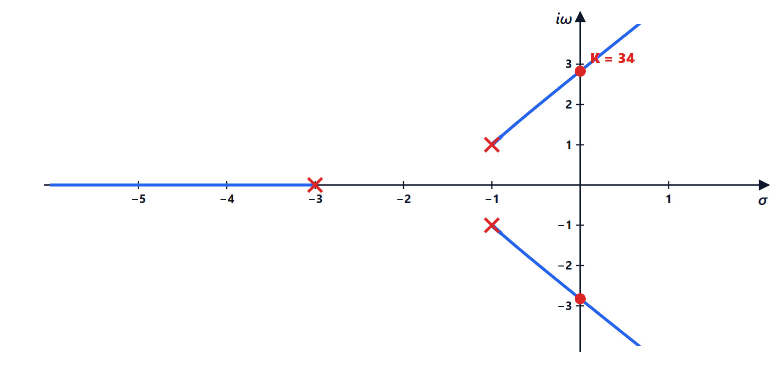
Characteristic equation:  . Stable if all coefficients are positive: .
Coincident poles: zero discriminant,  ,
 ,
 . For
 the double root is
 : the breakaway on the left, on the stretch to the left of the zero. For
 the root is , between the two unstable poles: a breakaway in the right half-plane.
The locus is a circle centred at with radius  :
 are exactly
 and
 . ✓
Exercise 7. A stabilising zero
To the system 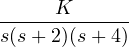 , unstable for
 , a zero at
 is added:
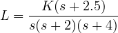 . Show that the closed loop is now stable for every
 .
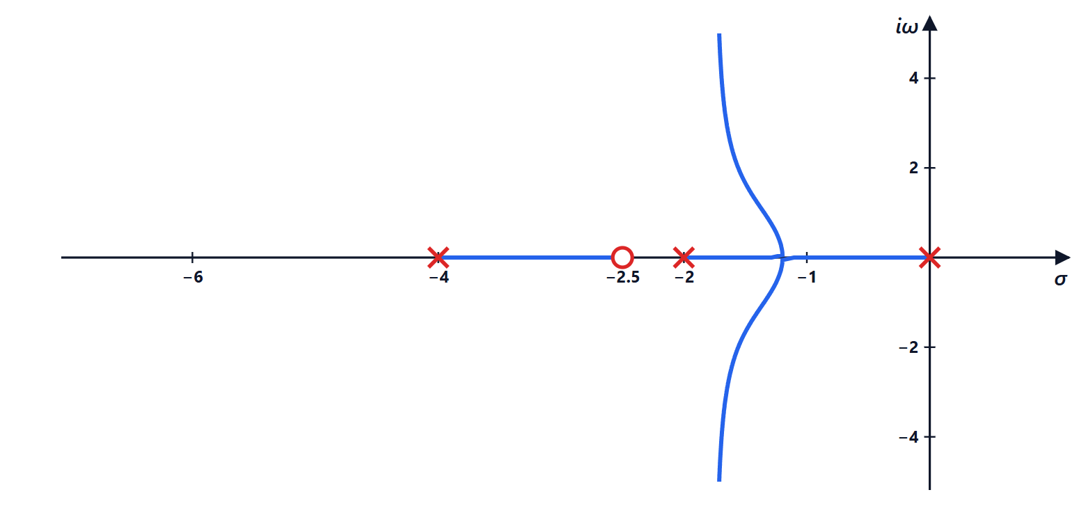
Result: vertical asymptotes with centroid  ; Routh always satisfied.
Solution
Asymptotes:  , angles , centroid
 . The branches going to infinity stay on the line
 , in the left half-plane.
Routh on  : all coefficients positive, and the third-order condition
 holds for every (it becomes
 ).
The zero is obtained with a PD controller,  , or in practice with a lead network (zero followed by a pole much further to the left, which leaves the picture almost unchanged).
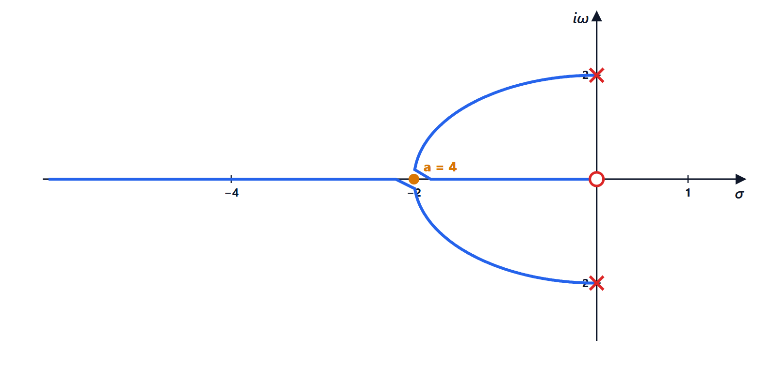
Exercise 8. The locus with respect to damping
The mass-spring-damper system  has adjustable damping
 . Sketch the path of the poles as
 varies and find for critical damping and for
 .
Result: the poles move on the circle  ; critical damping for
 ; for
 .
Solution
Characteristic equation  , rewritten as
 : a locus with poles
 and a zero at 0 (in-depth study).
As long as the poles are complex, their product is 4, so  : they lie on the circle of radius
 . With
 :
 . Critical damping
 for (poles coincident at ); for , poles
 .
Exercise 9. Design to an overshoot specification
The process  is controlled with a gain . Find for a 10 % overshoot and the corresponding settling time. Write the MATLAB and Python commands to check it.
Result:  ,
 ;
 s.
Solution
From the overshoot:  .
Characteristic equation  : ,
 , so
 and . Poles
 .
2 % settling time:  s, fixed by the real part , which a gain alone cannot move. For a faster system a zero is needed (lead network) to bring the locus further left.
Check in MATLAB: G = tf(1,[1 5 0]); stepinfo(feedback(17.9*G,1)). In Python: ct.step_info(ct.feedback(17.9*ct.tf([1],[1,5,0]),1)), which gives an overshoot of 10.0 % and a settling time of 1.42 s: the formula  is a conservative estimate, obtained from the exponential envelope.