Solved Z transform exercises: from difference equations to microcontroller code
Eleven exercises with solutions and graphs: transforms and inverse transforms, exponential filter, Fibonacci, stability, static gain, moving average, ZOH, Euler and Tustin, prewarping, digital PI written in C.
Exercises on the Z transform of the kind set in Mathematical Methods, Digital Signal Processing and Digital Control courses, in three levels: basic, with transforms and inverse transforms; intermediate, with difference equations, stability and frequency response; exam, with discretisations and the implementation of a digital controller down to the code. The result is given straight away; the full solution, with the graph, opens with a click. The tables are in the in-depth study linked at the top.
Basic level
Exercise 1. Multiplication by n
Compute the transform of  .
Result: 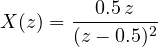 .
Solution
Start from  and use
 :

Double pole at 0.5: the sequence first grows (because of the factor  ) and then decays (because of
 ), with its maximum between
 and
 , where it equals 0.5.
Exercise 2. Inverting with partial fractions
Find the inverse transform of  and check the first samples by division.
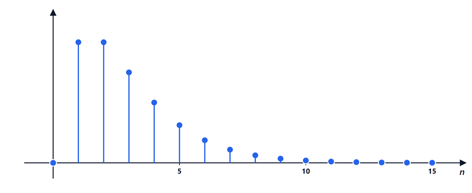
Result:  ;
 ,
 ,
 .
Solution
 , with
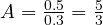 and
 .
Multiplying back by  :
 , so .
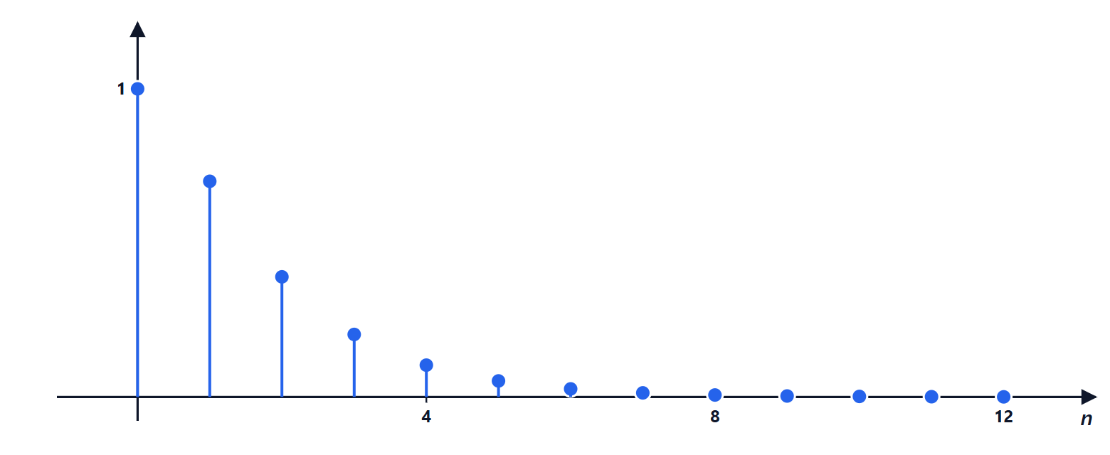
Check.  : it corresponds to
 . So , ,
 . From the formula:
 .
Exercise 3. The exponential filter and the step
A sensor is filtered with  . Find the transfer function, the step response and the number of samples after which the output exceeds 95 % of its final value.
Result: 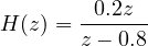 ;
 ; from sample
 .
Solution
Transforming:  , so
 . Static gain
 .
Step response:  .
 (residues: at 1 it is
 ; at 0.8 it is
 ). So
 .
95 %:  ,
 , i.e.
 . With 100 Hz sampling the filter responds in about 0.13 s: it is the trade-off between a clean signal and promptness.

Intermediate level
Exercise 4. The Fibonacci numbers
Solve with the Z transform  , with
 ,
 .
Result:  , with
 ,
 .
Solution
With the advance rule:  . With the initial values:
 , so
 .
Poles:  , i.e.
 (the golden ratio) and
 .
 , which gives Binet’s formula.
The pole  outside the unit circle makes the sequence grow exponentially; the pole
 , inside and negative, adds a small alternating correction that makes every term an integer. For large ,
 :
 , and
 .

Exercise 5. Stable or unstable
Determine the stability of the systems  and
 . For the second, how many samples does one oscillation last?
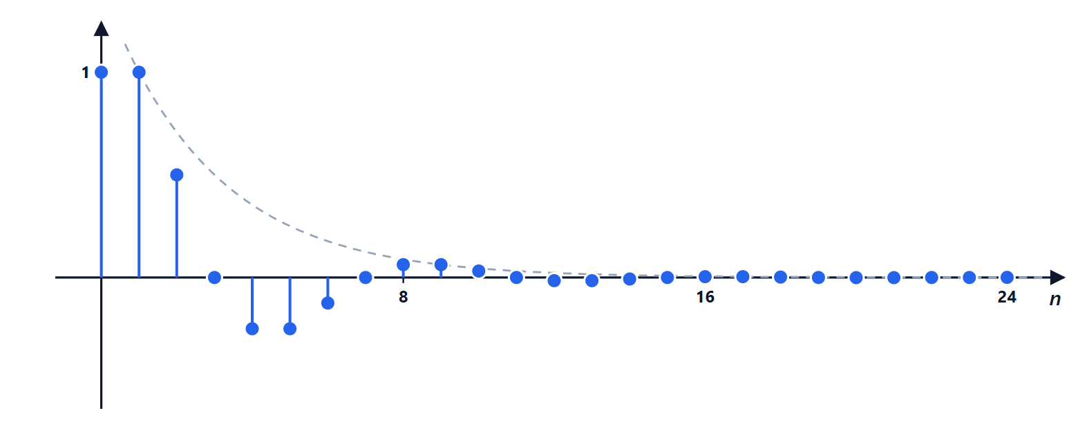
Result: the first is unstable (pole 1.1); the second is stable (poles  , modulus 0.707) and oscillates with a period of 8 samples.
Solution
First.  : pole at 1.1, outside the circle. The impulse response
 grows by 10 % at every sample.
Second. 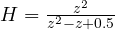 . Poles:
 . Modulus
 : stable. Angle
 : a full turn (
 ) takes
 samples.
Damping: after one period the amplitude is  , i.e. it drops to one sixteenth: the oscillation is barely visible.

Exercise 6. Final value and static gain
A discrete system has 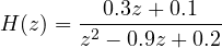 . Find the steady-state value of the unit step response.
Result: 1.33.
Solution
Poles:  , i.e.
 and
 , inside the circle: the final value exists.
With the step  :
 .
The static gain of a discrete system is  , as that of a continuous one is
 :
 corresponds to
 in the map
 .
Exercise 7. The moving average in frequency
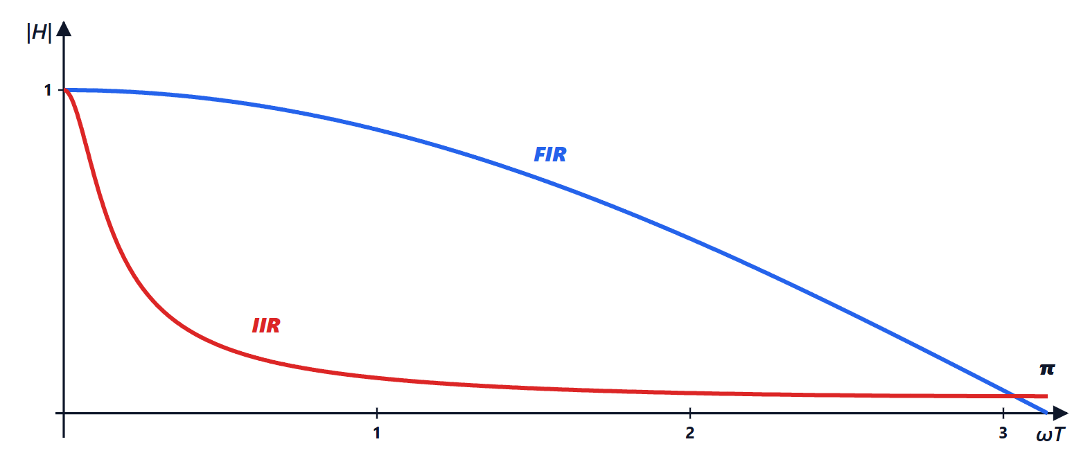
The filter  runs at
 kHz. Compute the gain at 0 Hz, at 250 Hz and at 500 Hz, and the delay it introduces.
Result: 1; 0.707 (−3 dB); 0; a delay of half a sample, 0.5 ms.
Solution
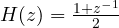 . With
 :
 .
Magnitude  , with
 : at 0 Hz it is 1; at 250 Hz
 ; at 500 Hz (Nyquist)
 .
Phase  , linear: all frequencies are delayed by
 ms. Symmetric FIR filters always have linear phase, and therefore do not distort the waveform.
Exam level
Exercise 8. Discretising a process with ZOH
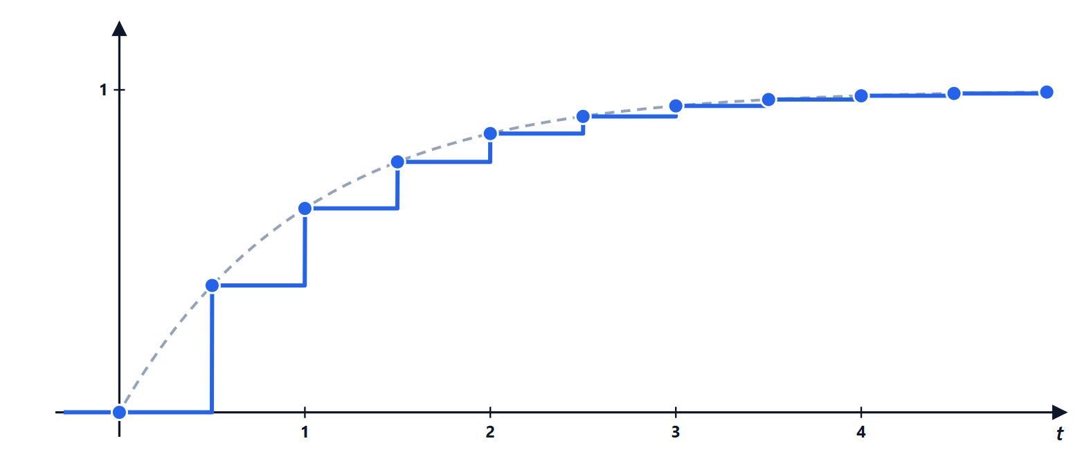
The process  is driven by a D/A with hold, with
 s. Find
 and check that, for a step, the samples coincide with the continuous response.
Result: 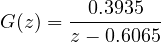 .
Solution
Formula of the in-depth study with  :
 .
Step response:  , whose inverse transform gives
 : exactly the continuous response
 at the instants
 . ZOH is exact for piecewise-constant inputs, because that is precisely what the D/A produces.
Exercise 9. Euler versus Tustin
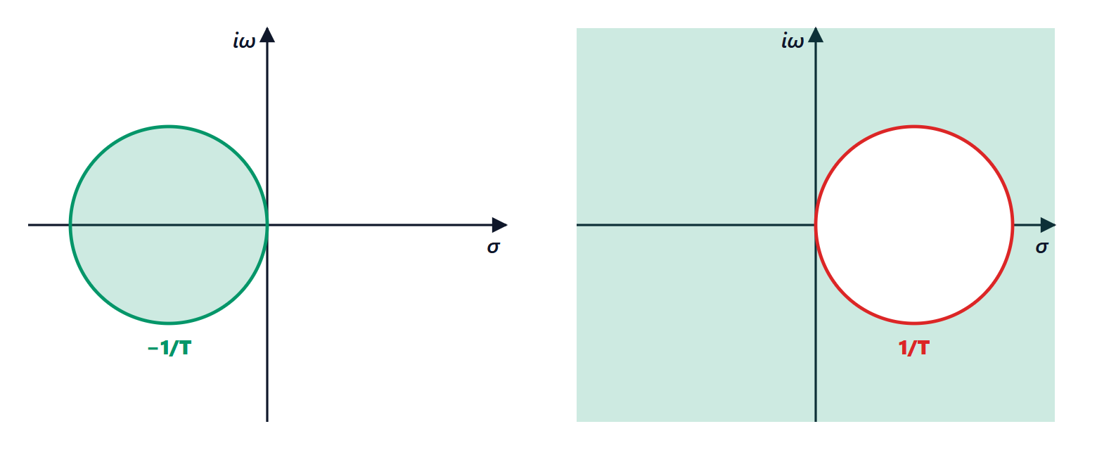
A controller has a pole at  . With
 s, where does the pole end up when discretising with forward Euler and with Tustin? And with ZOH?
Result: Euler  (unstable); Tustin
 (stable); ZOH
 .
Solution
Forward Euler:  . Outside the circle: a stable pole has become unstable, because
 .
Tustin:  . Stable, but negative: it introduces an oscillation at the Nyquist frequency that the continuous system did not have.
ZOH (exact correspondence):  .
Moral: with poles that are fast compared with the sampling the approximate methods give very different results. The practical rule is to sample at least 10-20 times faster than the fastest dynamics to be controlled.
Exercise 10. Tustin with prewarping
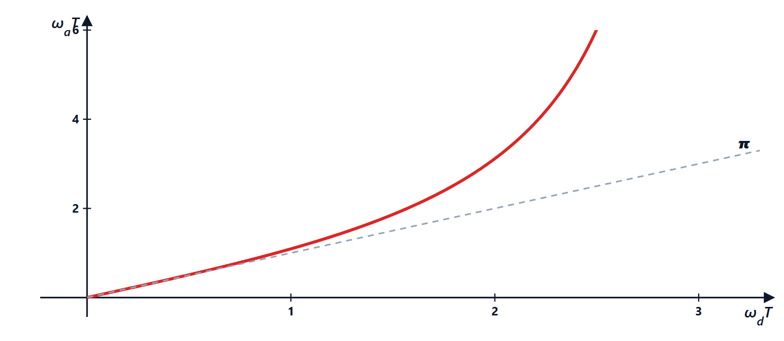
A digital low-pass filter with a cut-off frequency of 1 kHz, sampled at 4 kHz, is to be obtained with Tustin from a continuous prototype. At what frequency should the prototype be designed?
Result: at  rad/s (1273 Hz) instead of 6283 rad/s (1000 Hz).
Solution
Desired digital angular frequency:  ,
 , so
 .
With the Tustin warping,  corresponds to
 rad/s, i.e. 1273 Hz.
If the prototype were designed at 1000 Hz without correction, the digital filter would cut off at  Hz, 15 % lower.
In MATLAB: c2d(H, T, 'tustin') with the option c2dOptions('PrewarpFrequency', 2*pi*1000); in Python, scipy.signal.bilinear after scaling the prototype, or control.sample_system(H, T, method='tustin', prewarp_frequency=2*pi*1000).
Exercise 11. From the continuous PI to the microcontroller code
A PI controller  , with
 and
 s
 , must run on a microcontroller with
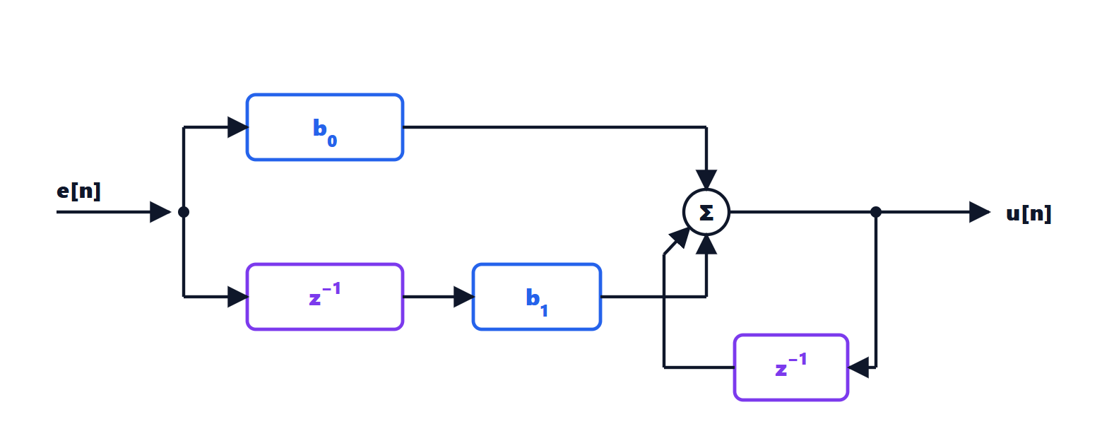
 ms. Discretise it with Tustin, write the difference equation and the code.
Result:  .
Solution
With  :
 . So

with  and
 .
From  :
 . Each
 is a variable that keeps the value of the previous step. In C, run by a periodic interrupt every 10 ms:
static float u_prev = 0.0f, e_prev = 0.0f;
const float b0 = 2.05f, b1 = -1.95f;

float pi_step(float setpoint, float measure)
{
    float e = setpoint - measure;
    float u = u_prev + b0 * e + b1 * e_prev;
    if (u > 10.0f) u = 10.0f;            /* actuator saturation */
    if (u < -10.0f) u = -10.0f;
    u_prev = u;                           /* z^-1 on the output */
    e_prev = e;                           /* z^-1 on the error */
    return u;
}
Saturating  and saving the already-limited value in
u_prev is a simple anti-windup protection: the integrator does not keep growing when the actuator is at its limit. This is exactly the scheme that in car ECUs controls engine idle speed, turbo boost pressure or the torque of an electric motor.