Partial differential equations: waves, heat and separation of variables
The three classic equations, d'Alembert's solution, the vibrating string with normal modes and Fourier series, the heat equation and diffusion times, Laplace's equation.
The differential equations of Analysis 2 had a single independent variable, time. But a signal travelling along a cable, heat spreading in a heat sink, the potential inside a semiconductor device depend on time and space. They call for partial differential equations (PDEs). In this lesson we look at the three classic equations, the method of separation of variables with the vibrating string and the heat equation, and the link with Fourier series.
The three classic equations
| Type | Equation | Phenomena |
|---|---|---|
| hyperbolic |  (waves) | vibrating strings, sound, electromagnetic waves, signals on transmission lines |
| parabolic |  (heat) | heat conduction, carrier diffusion in semiconductors |
| elliptic |  (Laplace) | electrostatic potential, steady-state temperature |
A unique solution needs boundary conditions (what happens at the edges of the domain) and, for equations involving time, initial conditions.
The wave equation and d’Alembert’s solution
For an infinite string, the equation  has the general solution

for any functions  and
 (differentiate twice to check).
 is a shape travelling right at speed
 without distortion,
 one travelling left. With initial conditions
 and
 one gets
 : the initial shape splits into two halves moving in opposite directions.
On transmission lines the voltage obeys the same equation, with 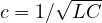 (inductance and capacitance per unit length): that is why fast signals on printed circuit boards must be treated as waves, with reflections at the ends if the impedance is not matched.
Separation of variables: the vibrating string
A string of length  fixed at both ends:
 . Look for solutions of the form
 . Substituting into the equation and dividing by
 :
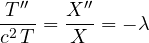
The left side depends only on  , the right side only on
 : they can be equal for every and only if both equal a constant. The PDE splits into two ordinary equations.
The eigenvalues
 with
 . For
 the only solution is zero. For
 ,
 :
 gives
 ,
 gives
 , that is

Only a discrete sequence of shapes is allowed: the normal modes.
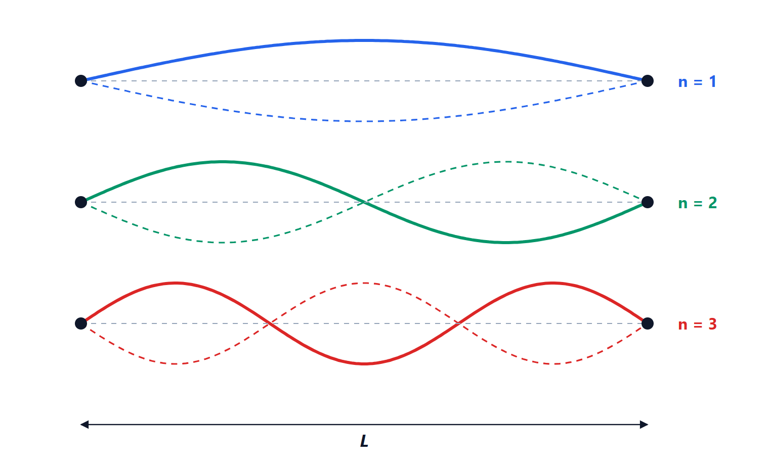
For each mode,  gives a harmonic oscillation with angular frequency
 . The frequencies are integer multiples of the fundamental
 : they are the harmonics of the lesson on Fourier series. It is the physics of every string instrument: halving the length (pressing the fret halfway up a guitar neck) doubles the frequency, one octave higher.
The general solution
By linearity, a sum of solutions is still a solution:

The coefficients come from the initial conditions, and here the Fourier series returns: with the string held still in an initial shape  , we need
 , so the
 are the coefficients of the sine series of
 :
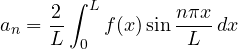
Plucking the string at a different point changes the coefficients, that is the weight of the harmonics, and so the timbre: that is why a guitar sounds different plucked near the bridge or in the middle.
The heat equation
A bar of length with its ends held at zero temperature and an initial distribution :  . Separation of variables gives the same spatial modes, but the time equation is now first order:
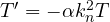 , with a decaying exponential solution. So

Two important remarks:
- there are no oscillations: the temperature decays towards equilibrium;
- the higher modes die out much faster (the factor is
 ): after a short time only the first mode remains, half a sine wave. Heat smooths out the irregularities of the initial distribution.
The characteristic time is  , proportional to the square of the length. For aluminium
 m²/s: a 10 cm bar settles in about
 s, a 1 m bar in about 17 minutes. Doubling the distance heat must travel quadruples the time: one of the golden rules of thermal design.
Laplace’s equation
In steady state the heat equation becomes . Separation of variables on a rectangle gives solutions like  ; on a disc, in polar coordinates,
 . The solutions are the harmonic functions of the lesson on complex functions, and this is where conformal mappings become useful: they take a complicated domain to a simple one where the solution is known.
When the geometry is too complicated for any analytical method, one turns to numerical methods, finite differences or finite elements, the subject of the Numerical Analysis course.