Floating-point arithmetic, errors, conditioning and stability
The IEEE 754 standard and machine epsilon, catastrophic cancellation with examples, condition number, stable and unstable algorithms.
Numerical analysis studies how to solve mathematical problems (equations, systems, integrals, differential equations) on a computer when an exact formula does not exist or cannot be used. The first step is to understand what a computer calculates with: not real numbers, but a finite set of floating-point numbers. This is where rounding errors come from, along with the difference between a well-conditioned problem and a stable algorithm.
Floating-point numbers
A computer represents a real number as

with a sign, a mantissa (significand) of  binary digits and an exponent
 in a limited range. The IEEE 754 standard, used by every modern processor, provides:
| Format | Total bits | Mantissa | Exponent | Decimal digits | Machine epsilon  |
|---|---|---|---|---|---|
| single (float) | 32 | 23 + 1 | 8 | about 7 |  |
| double | 64 | 52 + 1 | 11 | about 16 |  |
The leading bit of the mantissa is always 1 and is not stored (the “hidden bit”), hence the “+ 1”.
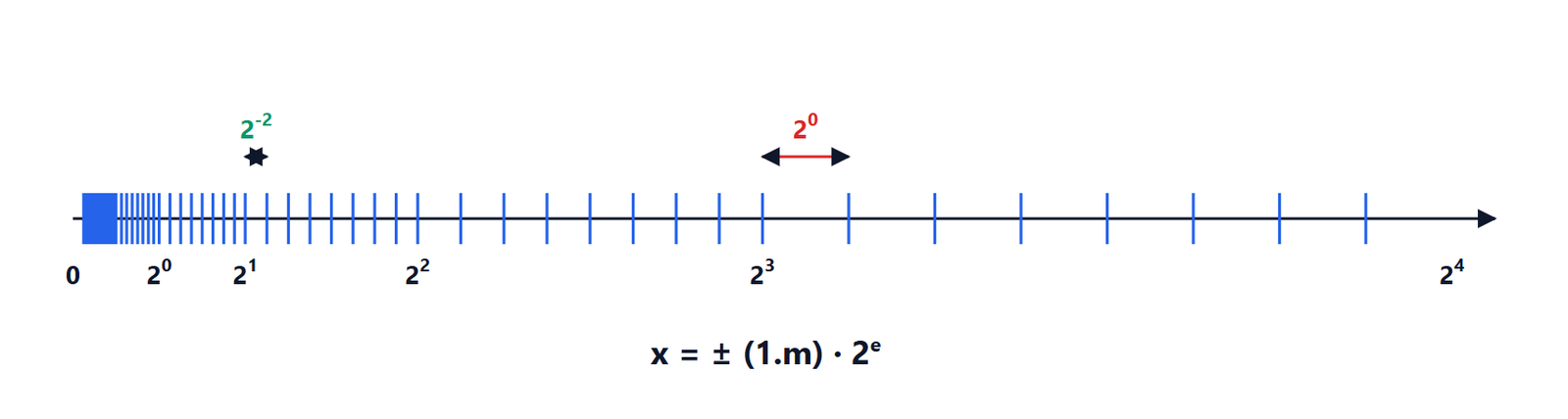
Machine epsilon is the gap between 1 and the next representable number. Every real  in the representable range is rounded to the nearest one, with a relative error of at most
 :

And every arithmetic operation has the same error:  .
Typical surprises.
 cannot be represented exactly in binary (like
 in decimal), so
 in double precision gives
 . Never compare floating-point numbers for exact equality: use
 .
- In single precision
 : beyond
 not every integer is representable.
- There are special values:
 (for example
 ) and NaN, “not a number” (for example
 ), which propagate through calculations instead of stopping the program.
Catastrophic cancellation
Subtracting two nearly equal numbers is the most dangerous operation. If  and
 have 16 correct digits and agree in the first 12, the difference has only 4: the rest is rounding noise.
Example: the quadratic equation.  has roots of about
 and
 . The textbook formula for the small root,
 , subtracts two nearly equal numbers and in double precision gives about
 : a 25% error. The fix is to rewrite the formula: compute the large root first, with no cancellation, then the small one from
 , that is
 , exact.
Example:  for small . With
 , the rounded
 is exactly 1 and the result is 0, while the true value is
 . Rewriting
 makes the calculation accurate. Libraries provide dedicated functions, such as expm1 and log1p, precisely for these cases.
Conditioning of a problem
Conditioning measures how much the exact result of a problem changes when the data are slightly perturbed. For a function  , the relative condition number is
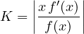
the relative error in the result is about  times that in the data. If is large the problem is ill-conditioned: even a perfect calculation on rounded data gives unreliable results. It is a property of the problem, not of the algorithm.
For linear systems  the condition number is
 . If
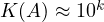 , about
 significant digits are lost: with
 in double precision only 4 reliable digits remain. The Hilbert matrix
 of order 10 has
 : the classic example of a system that is almost impossible to solve on a computer although it is invertible.
Stability of an algorithm
An algorithm is stable if it does not amplify rounding errors more than the problem itself already does. The same well-conditioned problem can be solved with a stable or an unstable algorithm, as in the quadratic equation example.
An unstable algorithm. The integrals  satisfy
 , with
 . Running the recurrence forwards, the initial error (of the order of
 ) is multiplied by
 : with
 ,
 , and the result is completely wrong, even negative, although
 always lies between 0 and 1. Running it backwards,
 , starting from any value at a large
 , the error is divided by at each step and the result is accurate.
A rule of thumb
Final error  condition number
 machine epsilon, if the algorithm is stable. In the following lessons, for each method we will ask three questions: does it converge, how fast, and is it stable. The famous case of the Ariane 5 rocket, which exploded in 1996 because a 64-bit floating-point number was converted into a 16-bit integer that could not hold it, is a reminder that these details are not academic.