Root finding: bisection, Newton, secant and fixed point
Bisection, Newton's method with proof of quadratic convergence, the secant method, fixed-point iteration, Newton for systems and SPICE.
Finding where a function is zero is one of the most frequent problems: the operating point of a diode in a circuit (where the diode’s exponential equation meets the load line), the frequency at which a filter attenuates by 3 dB, the launch angle to hit a target. For almost every nonlinear equation there is no formula, so one proceeds by iteration: start from an estimate and improve it until it is accurate enough.
The bisection method
If  is continuous on
 and
 and
 have opposite signs, by the intermediate value theorem of Analysis 1 there is at least one root. Bisection halves the interval at each step:
- compute the midpoint
 ;
- if and
 have opposite signs the root is in
 , otherwise in
 ;
- repeat until the interval is smaller than the tolerance.
After  steps the interval is
 wide. Going from an interval of 1 to a tolerance of
 takes 20 steps (
 ). The method is slow but it always converges, and the error bound is guaranteed. It gains one decimal digit every 3.3 steps or so.
Newton’s method
The idea is to replace the function with its tangent line and take as the new estimate the point where the tangent crosses the axis:
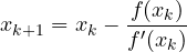
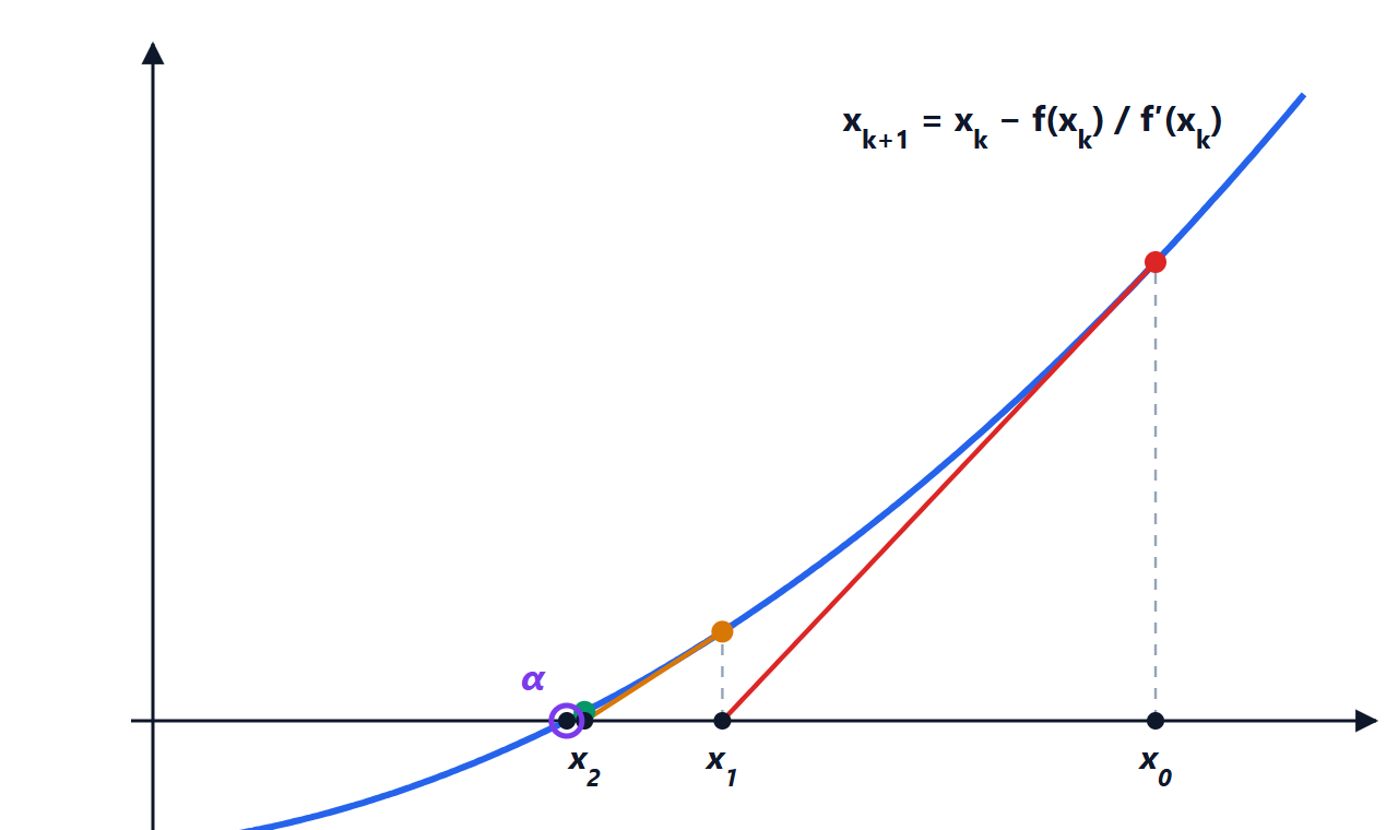
 , the tangent to the graph at crosses the axis at
 ; the tangent at gives
 , and so on. The estimates approach the root α very quickly.
Example: the square root. With  the formula becomes
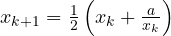 , the Babylonian method. For
 starting from
 (as in the figure): 1.8333; 1.4621; 1.41500; 1.4142138; 1.41421356237311. The correct decimal digits go 0, 1, 3, 6, 13: they roughly double at every step.
Proof of quadratic convergence
Let  be the root and
 the error. Expanding with Taylor around
 , evaluated at :

Dividing by  and using the definition of the iteration,
 :
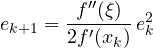
The new error is proportional to the square of the old one: if  ,
 is of the order of
 . This is quadratic convergence, far faster than bisection, which is linear.
Newton’s limits
- It needs the derivative, which is not always available.
- Convergence is guaranteed only when starting close enough to the root. Far away, the tangents can send the estimate anywhere or make it oscillate: with
 and
 the estimates diverge.
- If
 (a double root) convergence becomes only linear.
In practice the two methods are combined: bisection until the interval is small, then Newton to finish in a few steps. This is what functions such as MATLAB’s fzero or SciPy’s brentq do.
The secant method
When the derivative is not available it is approximated by the difference quotient of the last two estimates:

Convergence is superlinear, of order 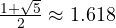 (the golden ratio), and each step needs only one evaluation of : it is often more efficient than Newton.
Fixed-point iteration
Every equation  can be rewritten as
 , and a fixed point sought with
 . It converges if
 near the solution: the error is multiplied by about
 at each step.
Example.  : starting from any value and repeatedly pressing the cosine key of a calculator (in radians) you reach 0.739085…, because
 near the solution. Newton itself is a fixed-point iteration with
 , which has
 : that is why it converges faster.
Nonlinear systems
For a system  of equations in unknowns, Newton generalises with the Jacobian matrix of Analysis 2:

at each step a linear system is solved. It is the heart of SPICE: for a circuit with diodes and transistors, the simulator linearises the components around the current estimate and solves the linear system, repeating until the voltages stop changing. When a simulation “fails to converge”, it is Newton failing to find the solution from the initial guess.
Stopping criteria
Stop when the difference between two successive estimates is below a tolerance,  , or when the residual
 is small enough, and in any case after a maximum number of iterations, so as not to get stuck if the method does not converge. A small residual alone is not enough: if the function is very flat near the root,
 can be tiny even far from the solution.





