Taylor and Maclaurin expansions: polynomials, remainder and limits
The Taylor polynomial, Peano and Lagrange remainders, the expansions to know, computing limits with Taylor and applications to linearisation.
The tangent line approximates a function near a point. The Taylor polynomial does the same with a parabola, a cubic, a polynomial of any degree, and the approximation improves with every extra degree. It is the most powerful tool of first-year calculus for limits, and the one calculators use to compute sines and exponentials.
The Taylor polynomial
If  is
 times differentiable at
 , its Taylor polynomial of order is

It is the only polynomial of degree  with the same value and the same first derivatives as at . With
 it is called the Maclaurin polynomial.
The remainder
The error  can be written in two ways:
- Peano remainder:
 , that is the error is negligible compared with
 as
 . This is what you need for limits;
- Lagrange remainder:
 for some
 between and
 . This is what you need to estimate the error numerically.
The symbol  (“little o of g”) denotes a quantity that, divided by
 , tends to 0. Useful rules:
 ,
 ,
 if
 .
Expansions to know (x → 0)
 |  |
 |  |
 |  |
 |  |
 |  |
 |  |
 |  |
 | 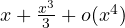 |
Expansions of composite functions come by substitution:  ,
 .
Computing limits with Taylor
Expand numerator and denominator up to the first term that does not cancel.


In the second example first-order equivalences give  and l’Hôpital would need four derivatives: Taylor takes two lines. The practical rule is to push the expansion up to the order of the denominator.
Other uses
- Nature of stationary points: if
 and the first non-zero derivative has order , for even the point is an extremum (a minimum if
 ), for odd it is an inflection point.
- Numerical computation:
 , with a Lagrange error below
 .
- Linearisation: in electronics the “small-signal” models of the diode and the transistor are the first-order expansion of the exponential characteristic around the operating point, and the second- and third-order terms are the harmonic distortion.

