Partial derivatives, gradient, differentiability and the tangent plane
Partial derivatives and the gradient, why they are not enough, differentiability and the tangent plane, directional derivative and steepest ascent, the chain rule and the Hessian.
In one variable the derivative tells how fast a function grows. In several variables the question becomes: how fast does it grow moving in a given direction? The answer leads to partial derivatives, the gradient, the tangent plane and differentiability, which is the right notion for saying that a function is “smooth”.
Partial derivatives
The partial derivative with respect to  is computed by holding
 fixed and differentiating as in Analysis 1:

Geometrically it is the slope of the curve obtained by cutting the graph with the plane  . Example:
 has
 and
 .
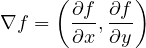
The vector of partial derivatives is the gradient:
Partial derivatives are not enough
In one variable, differentiable implies continuous. In several variables it does not: the function  , extended by 0 at the origin, has both partial derivatives zero at
 (along the axes it is always 0), but it is not even continuous there. Partial derivatives look at only two directions, while the behaviour around a point depends on all of them.
Differentiability and the tangent plane
 is differentiable at
 if it can be approximated by a linear function with an error that goes to zero faster than the distance:

Geometrically: near the point the graph cannot be told apart from a plane, the tangent plane

Differentiable implies continuous and having every directional derivative. The practical test: if the partial derivatives exist and are continuous near the point, the function is differentiable (total differential theorem). All functions built from elementary operations are, where the derivatives are continuous.
Example. The tangent plane to  at
 :
 ,
 , so
 .
Directional derivative
The derivative in the direction of the unit vector  is

and, if is differentiable, the gradient formula holds:

Proof and consequences
From the definition of differentiability with  :
 ; dividing by
 and taking the limit gives the formula. From the cosine three key facts follow:
- the directional derivative is largest in the direction of the gradient (
 ) and equals
 : the gradient points in the direction of steepest ascent;
- it is smallest,
 , in the opposite direction;
- it is zero in directions perpendicular to the gradient.
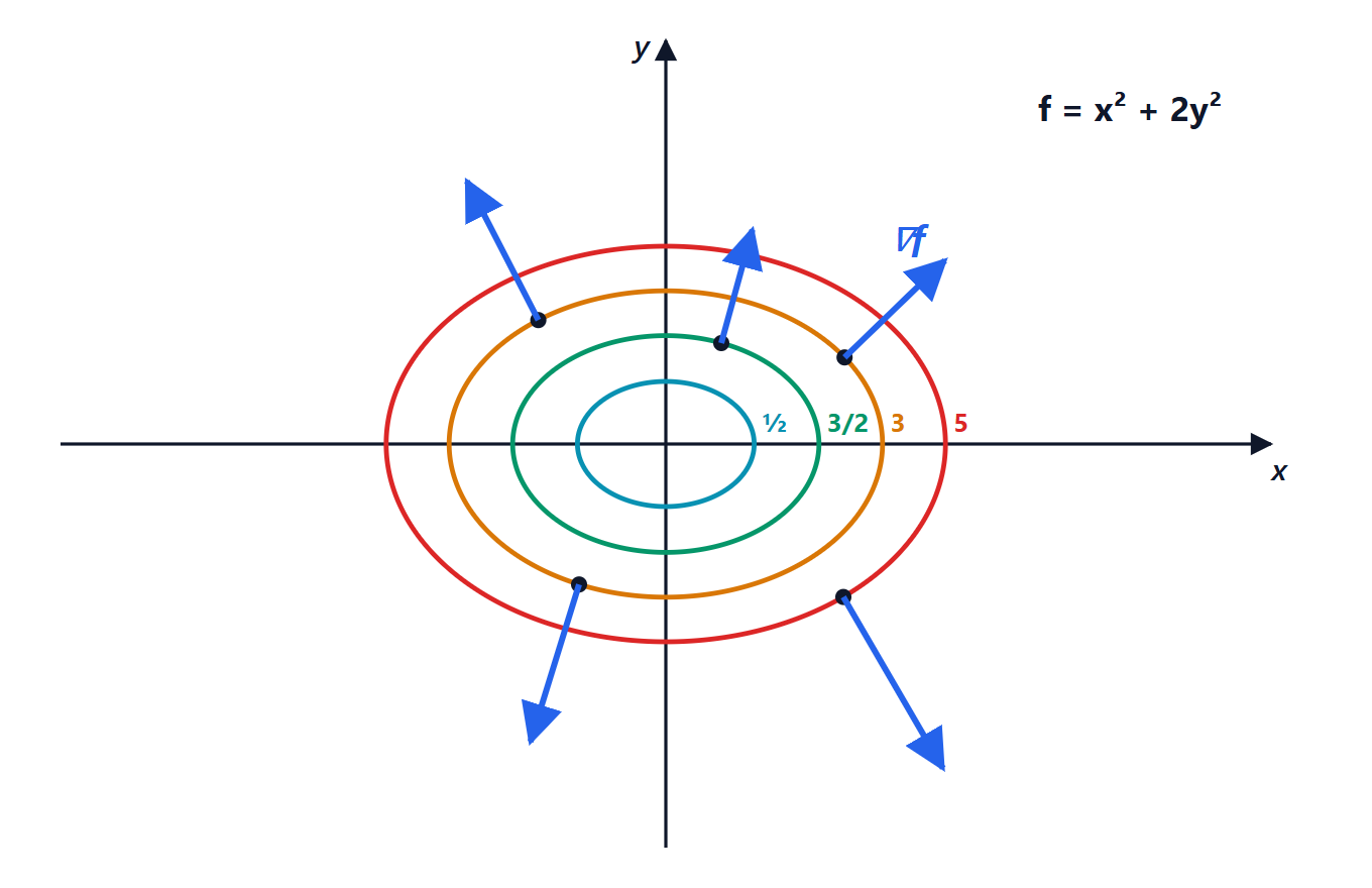
 and the gradient at a few points: it is always perpendicular to the level curve through the point and points towards increasing values. Where the curves are closer together the gradient is longer.
Along a level curve is constant, so the derivative in the tangent direction is zero: the gradient is perpendicular to the level curves. That is why electric field lines  cross equipotential surfaces at right angles, and why water runs down the steepest slope, perpendicular to the contour lines.
The chain rule
If  and
 describe a curve, the composite function
 has derivative

Example. The temperature on a plate is  °C (with
 in metres) and an ant moves along
 metres, with in seconds. At time
 ,
 and
 : the ant feels the temperature drop by
 °C per second.
More generally, for  the derivative is the Jacobian matrix, with the partial derivatives of each component along the rows, and the chain rule says that the Jacobian of a composition is the product of the Jacobians. It is the bridge between Analysis 2 and Geometry and Algebra: differentiating means approximating with a linear map.
Second derivatives
Differentiating again gives the second derivatives  , collected in the Hessian matrix. Schwarz’s theorem guarantees that, if the mixed second derivatives are continuous, the order does not matter:
 , and the Hessian is symmetric. We will use it in the next lesson to classify maxima, minima and saddle points.