Curves, line integrals and conservative fields
Parametric curves and length, the integral of a function and the work of a field, conservative fields and potential, irrotational fields, the wire counterexample and finding the potential.
A curve in space is the path of a moving point. Along a curve you can integrate two different things: a scalar function (to compute a length or a mass) or a vector field (to compute work). This lesson introduces both integrals and arrives at conservative fields and potentials, which in Physics 2 will become the electric potential.
Parametric curves
A curve is a function  ,
 . The vector
 is tangent to the curve and, if
 is time, it is the velocity. The curve is regular if
 is continuous and never zero.
Examples. The circle  ,
 . The helix
 , the shape of a spring and a screw thread. The graph of
 is the curve
 .
The length of a curve
Approximating the curve with a polygonal line and taking the limit, the length is the integral of the speed:
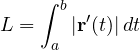
Example. One turn of the helix  :
 , so
 . It is the hypotenuse of a right triangle with legs
 (the circumference) and
 (the pitch): unrolling the cylinder, the helix becomes a straight line.
The length does not depend on how the curve is parametrised: travelling faster or slower does not change the road.
Line integral of a function
For a scalar function  (for example the linear density of a wire):
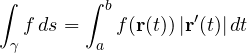
where  is the element of length. With
 you get the length back; with a density you get the mass of the wire. It does not depend on the direction of travel.
Line integral of a vector field: work
If  is a force, the work done along the curve
 is
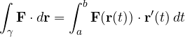
Only the component of tangent to the curve counts. Unlike the previous case, it changes sign if the direction is reversed.
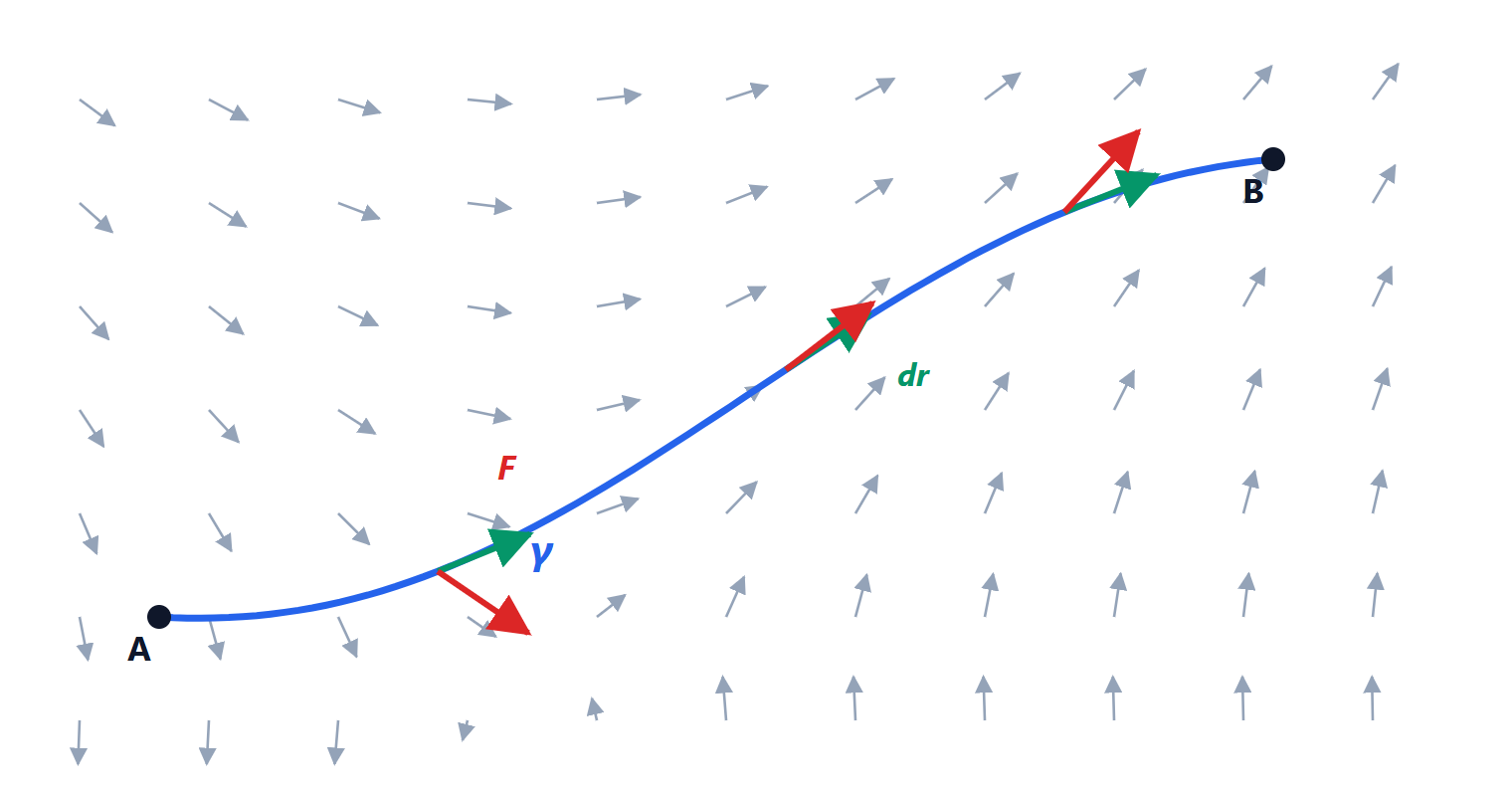 (grey and red arrows) and the curve from A to B with tangent vectors
 (green). The line integral adds up, point by point, the dot product of field and displacement: where they agree the contribution is positive, where they oppose it is negative.
Example.  along the unit circle anticlockwise:
 ,
 , dot product 1, integral . The field “turns” the same way as the curve and does positive work all the way round.
Conservative fields
A field is conservative if there is a function  , the potential, such that
 . (Physics often uses the opposite sign,
 , with
 the potential energy.)
Theorem. If , then for every curve from A to B
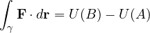
Proof
By the chain rule  . So the integral is
 , by the fundamental theorem of calculus.
Three equivalent properties follow (in a connected domain):
- has a potential;
- the integral between two points does not depend on the path;
- the integral around every closed curve is zero.
The field  of the previous example is not conservative: around a closed loop it gave , not zero.
How to recognise a conservative field
If  , then
 ,
 , and by Schwarz’s theorem
 . The condition

(an irrotational field; in three dimensions  ) is therefore necessary. It is also sufficient if the domain is simply connected, that is with no “holes” a closed curve could go around.
The classic counterexample. 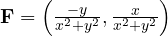 on the plane without the origin is irrotational, but its integral round the unit circle is . The hole at the origin breaks the equivalence. It is, up to constants, the magnetic field of a straight wire carrying a current: its integral round a closed curve counts how many times the curve goes round the wire, and that is Ampère’s law.
How to find the potential
Example.  . Check:
 , and the domain is the whole plane. Integrating
 in
 :
 . Differentiating in
 and comparing with
 :
 , so
 . The potential is
 , and the work from
 to
 is
 , whatever the path.