Linear maps: the associated matrix, kernel, image and the rank-nullity theorem
Definition and examples, the matrix of a map with rotations and the derivative, kernel and image, proof of the rank-nullity theorem and change of basis.
Linear maps are the functions of linear algebra: they turn vectors into vectors while respecting sums and multiples. Rotations, projections, derivatives and digital filters are all examples. In this lesson we see that every linear map between finite-dimensional spaces is represented by a matrix, introduce kernel and image and prove the rank-nullity theorem.
Definition
A function  between vector spaces is linear if

An immediate consequence:  . So
 , despite being called a “linear function” at school, is not linear in this sense: it is a line that does not pass through the origin.
Examples: rotation of the plane by an angle  ; projection of space onto a plane; the derivative, which sends a polynomial
 to
 and respects sums and multiples; a FIR digital filter,
 , which is linear in the input signal.
The matrix of a linear map
A linear map is determined by the images of the vectors of a basis. If  , by linearity

Placing the images  as columns gives a matrix
 , and
 . Conversely, every
 matrix defines a linear map from
 to
 . The columns of are the images of the basis vectors: that is the rule to remember.
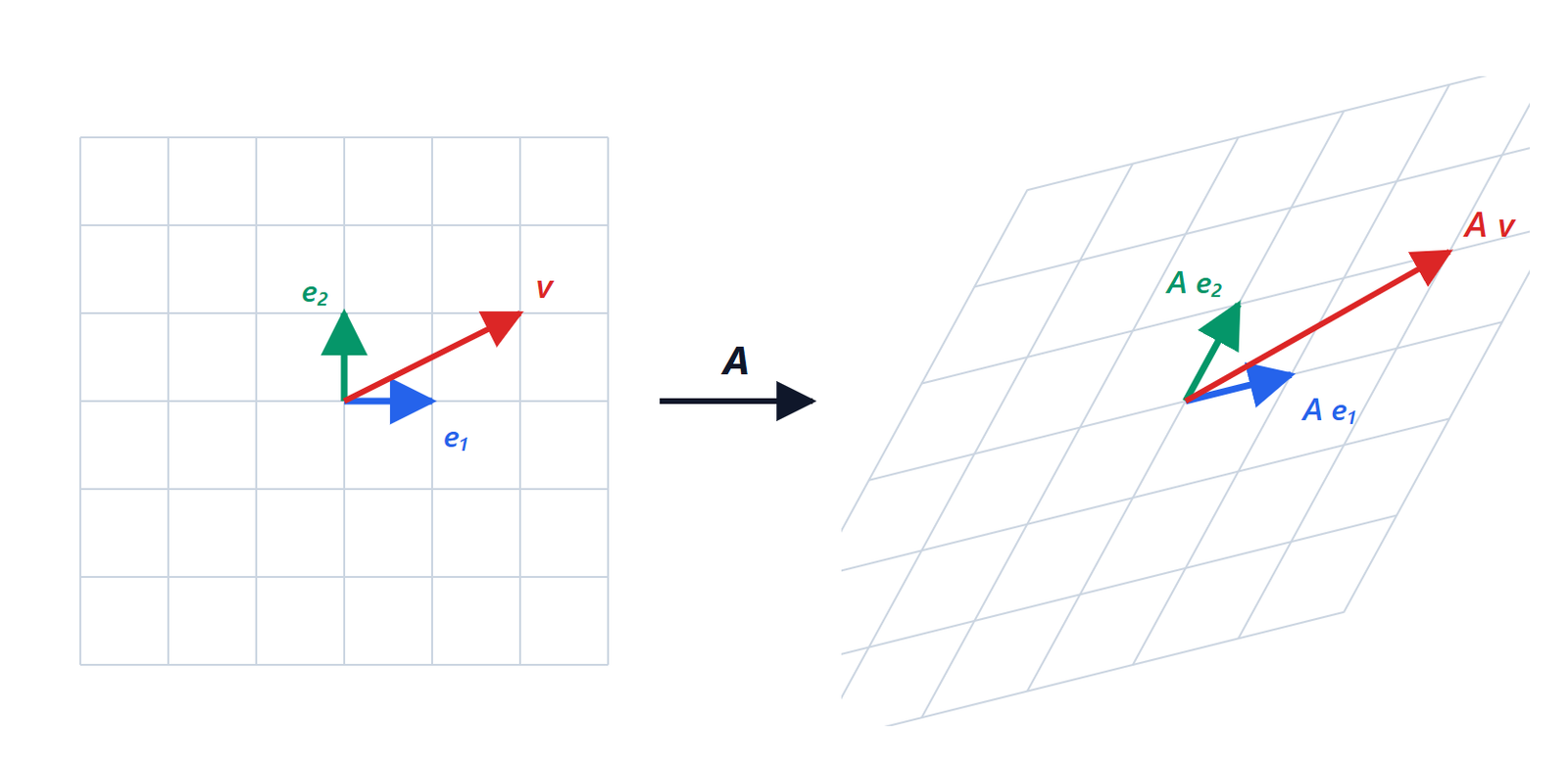
 and
 go (the columns of ) is enough to know where every vector goes:
 has, relative to
 , the same coordinates that
 has relative to
 .
Example: rotation. Rotating by ,  goes to
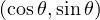 and
 goes to
 . So
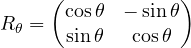
Composing two rotations,  : expanding the product gives back the addition formulas for sine and cosine, with no need to memorise them.
Example: the derivative. On  with basis
 :
 ,
 ,
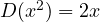 . The coordinates of these images are the columns:
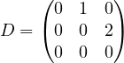
Differentiating  is the same as multiplying
 by
 : the result is
 , that is
 .
Kernel and image
- The kernel
 is a subspace of
 : for a matrix, it is the solution set of the homogeneous system
 .
- The image
 is a subspace of
 : for a matrix, it is the column space, and its dimension is the rank.
 is injective if and only if
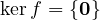 . Indeed
 is equivalent to
 , that is
 . is surjective if and only if
 .
The rank-nullity theorem
Theorem. If is linear and is finite-dimensional,

Proof
Let  be a basis of
 . Extend it to a basis of by adding
 , with
 . We show that
 is a basis of the image, so
 .
They span. Every is  , and
 because
 .
They are independent. If  , then
 , so
 is in the kernel and can be written as
 . But then
 is a zero combination of vectors of a basis of : all coefficients are zero, in particular the
 .
For an matrix of rank  the theorem says
 : it is the number of free parameters in the Rouché-Capelli theorem, which is now fully proved.
Consequences. A linear map from to itself is injective if and only if it is surjective (if and only if it is invertible). A map from  to
 cannot be injective: the kernel has dimension at least 1. One from to cannot be surjective.
Change of basis
The matrix of a map depends on the chosen basis. If  is the matrix whose columns are the vectors of a new basis (written in the old basis), coordinates change by
 , and the matrix of the map
 in the new basis is

Two matrices related in this way are called similar: they represent the same transformation seen from two different frames. They have the same determinant, rank, trace and eigenvalues. Choosing the right basis to make  as simple as possible, ideally diagonal, is exactly the topic of the next lesson.