Matrix rank and the Rouché-Capelli theorem
Row and column rank, computing it with Gauss and with minors, proof of the Rouché-Capelli theorem, the structure of solutions and systems with a parameter.
Rank is the number that says “how much independent information” a matrix holds. It ties together the three previous lessons (systems, determinant, vector spaces) and leads to the Rouché-Capelli theorem, which answers once and for all the question: when does a linear system have solutions, and how many?
Definition
The rank of a matrix  ,
 , is the largest number of linearly independent columns, that is the dimension of the space spanned by the columns. An important result is that it equals the largest number of independent rows: row rank and column rank are the same. So for an
 matrix
 .
How to compute it
With Gauss. Elementary row operations do not change the rank (they do not change the space spanned by the rows). The rank is therefore the number of pivots in the echelon form, that is the number of non-zero rows.
With minors. A minor of order  is the determinant of a
 submatrix. The rank is the largest order of a non-zero minor. To avoid trying them all one uses the bordering theorem (Kronecker’s): if a minor
 of order is non-zero and all minors of order
 that contain it (“bordered” minors) are zero, then the rank is .
Example.

Two pivots:  . Indeed the third row of is the sum of the first two, and the second column is twice the first.
The Rouché-Capelli theorem
Theorem. The system  , with
 unknowns, has solutions if and only if

In that case, calling  the common rank, the solutions depend on
 free parameters. In particular the solution is unique if and only if
 .
Proof
 is a combination of the columns of . The system has a solution if and only if
 is a linear combination of the columns of , that is if and only if lies in the space spanned by the columns. Then adding as a column does not increase the dimension of that space:
 . If instead is not a combination of the columns, adding it raises the rank by one.
For the number of parameters: if  is a solution, all the others are
 with
 (the difference of two solutions solves the homogeneous system). The solution space of the homogeneous system, the kernel of , has dimension , as we will prove with the rank-nullity theorem in the lesson on linear maps.
In short, the structure of all solutions is:

One particular solution plus the general solution of the homogeneous system: the same structure you meet in the linear differential equations of Analysis 2 and in circuits (forced response plus natural response). It is no coincidence: they are all linear problems.
Systems with a parameter
Exam problems often ask to discuss a system as a parameter varies.
Example.
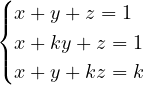
The determinant of the coefficient matrix, after subtracting the first row from the others, is that of a triangular matrix:
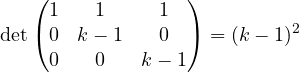
 :
 , rank 3 = number of unknowns, a single solution. From the second equation minus the first,
 , so
 ; from the third minus the first,
 , so
 ; finally
 . Solution
 .
 : all three equations become
 .
 , the solutions depend on
 parameters: a plane.
Had the right-hand side of the third equation been  instead of , for we would have had
 and
 : an inconsistent system.
Rank and invertibility
For a square  matrix the following are equivalent:
- is invertible;
- ;
 ;
- the columns (and the rows) of form a basis of
 ;
 has only the zero solution;
- has exactly one solution for every .
This list is one of the most used tools in the course: to prove one property it is enough to prove another.