The determinant: geometric meaning, Laplace expansion and Cramer's rule
Sarrus and Laplace, the determinant as area and volume, properties and Binet's theorem, computing with Gauss, invertibility, the adjugate and a proof of Cramer's rule.
The determinant is a number attached to every square matrix that sums up a key fact: whether the matrix is invertible or not. It also has a precise geometric meaning, which makes all its properties natural: it measures how much the matrix stretches areas and volumes. In this lesson we define it, see how to compute it and look at its uses, up to Cramer’s rule.
Order 2 and 3
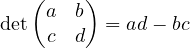
For order 3 you can use the rule of Sarrus: add the products of the three diagonals going down to the right and subtract those of the three going down to the left.

Careful: Sarrus works only for 3×3 matrices. Higher orders need Laplace expansion or Gaussian elimination.
The geometric meaning
The columns of  are the images of the basis vectors,
 and
 . The unit square built on
 is mapped to the parallelogram built on the columns of .
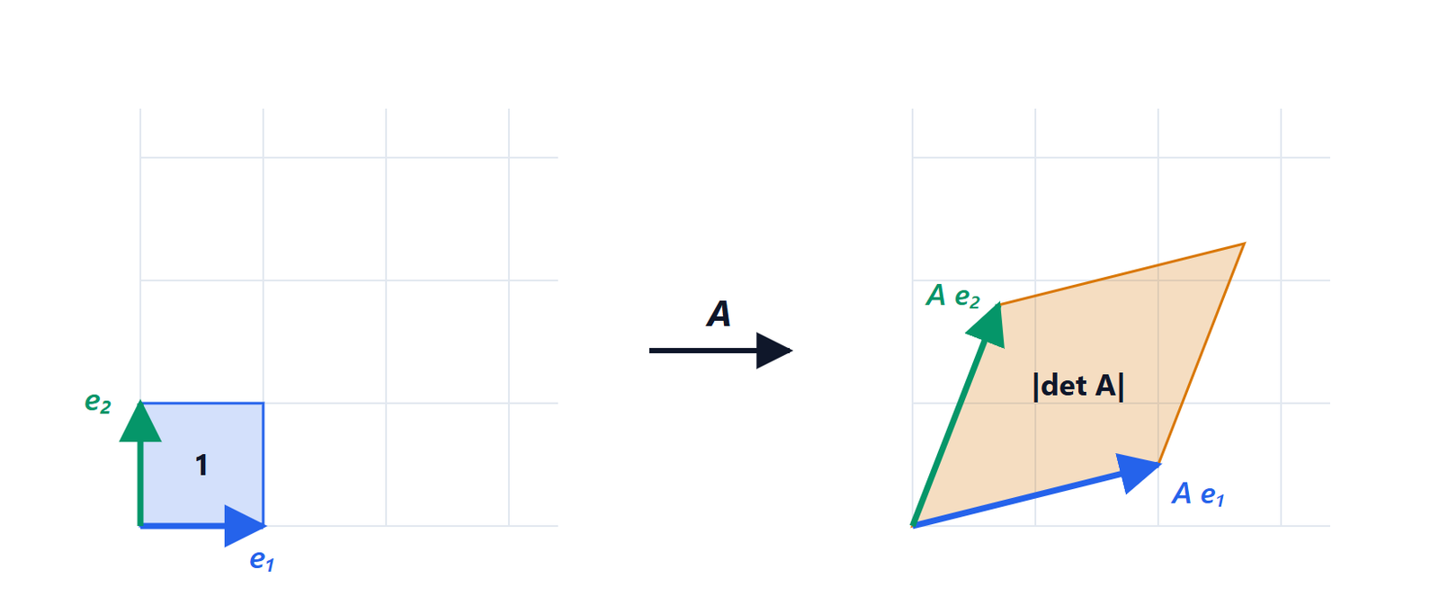 maps the square of area 1 to the parallelogram built on its columns. The area of that parallelogram is
 : here has columns
 and
 , and
 .
Proof in the 2×2 case
The parallelogram with sides  and
 has an area equal to the magnitude of the cross product of the two vectors seen in space with a zero third component:
 . So the area is
 . In three dimensions, likewise, is the volume of the parallelepiped built on the columns: it is the triple product of the lesson on vectors.
The sign gives the orientation: positive if the transformation keeps the sense of rotation (from  to
 anticlockwise), negative if it reverses it, as a mirror does. And if
 the parallelogram is flattened onto a line: the transformation loses a dimension and cannot be inverted.
Laplace expansion
For an  matrix, let
 be the submatrix obtained by deleting row
 and column
 . The cofactor is
 . Then, expanding along any row :
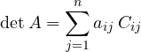
and the same holds along any column. Choose the row or column with the most zeros. The signs  follow the chessboard pattern starting with
 at the top left.
Example.

Properties
- Swapping two rows changes the sign of the determinant.
- Multiplying a row by
 multiplies the determinant by . Hence
 .
- Adding a multiple of one row to another does not change the determinant.
- If two rows are equal or proportional, or a row is zero, .
 : everything true for rows is true for columns.
- The determinant of a triangular matrix is the product of its diagonal entries.
- Binet’s theorem:
 .
Property 7 has an immediate geometric reading: applying  and then scales areas first by
 and then by
 . It follows that
 .
Computing with Gauss
Properties 1, 3 and 6 give the most efficient method: reduce the matrix to triangular form with elementary operations, multiply the diagonal and change sign once for each row swap. For a 10×10 matrix Laplace expansion takes millions of products, Gauss a few hundred.
Determinant and invertibility
Theorem. A square matrix is invertible if and only if  .
If is invertible, by Binet  , so . Conversely, if the inverse can be written explicitly with cofactors:
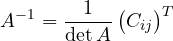
(the transpose of the cofactor matrix is called the adjugate). For 2×2 matrices we get back the formula from the lesson on matrices.
Cramer’s rule
If , the system  has the single solution

where  is the matrix with column replaced by
 .
Proof. Let  be the solution. In the matrix column is
 , a combination of the columns of . Since the determinant is linear in each column,
 splits into
 determinants: those with
 ,
 , in position have two equal columns and are zero. What is left is
 .
Example.  ,
 :
 ,
 ,
 .
Cramer is handy for 2×2 and 3×3 systems by hand, and for getting symbolic formulas (like voltage dividers in circuits), but with many unknowns it is far slower than Gauss.