Matrices: operations, the row-by-column product and the inverse
Why the row-by-column product is composition, properties and non-commutativity, special matrices and the transpose, the 2×2 inverse and computing it with Gauss-Jordan.
A matrix is a table of numbers, but above all it is a compact way of writing transformations and systems. In this lesson we cover matrix operations, why the row-by-column product is defined the way it is, special matrices and how to compute the inverse.
Definitions
An  matrix has
 rows and
 columns; the entry in row
 and column
 is written
 . If
 the matrix is square of order . Real matrices form the set
 .
Addition and multiplication by a scalar are done entry by entry, and they have the same properties as for vectors: is a vector space of dimension  .
The row-by-column product
If  is and
 is
 , the product
 is the
 matrix with
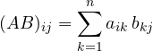
that is, the dot product of row of with column of . The number of columns of must equal the number of rows of .

Why it is defined this way
A matrix transforms a vector  into the vector
 . If we first apply and then , we get
 . Writing out the components:

The coefficient in brackets is exactly  : the matrix product is the composition of the transformations. It follows at once that the product is associative,
 , because composition of functions is.
The product is not commutative
In general  , even when both exist. Rotating by 90° and then reflecting in the
 axis does not give the same result as reflecting and then rotating. Other differences from numbers:
 does not imply
 or
 : for example
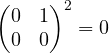 ;
- from
 you cannot “cancel” , unless is invertible.
Special matrices
- Identity
 : 1 on the diagonal, 0 elsewhere.
 .
- Diagonal: zeros off the diagonal. They multiply entry by entry along the diagonal, and their powers are trivial.
- Triangular, upper or lower: zeros below (or above) the diagonal. The echelon form of Gaussian elimination is upper triangular.
- Transpose
 : rows and columns swapped,
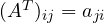 . We have
 (mind the order).
- Symmetric:
 . They appear everywhere, from covariance matrices to the stiffness matrices of structures, and have special properties we will meet with the spectral theorem.
The inverse matrix
A square matrix is invertible if there is  with
 . If it exists it is unique, and the system
 has the single solution
 .
We have  and
 . A matrix is invertible if and only if its determinant is non-zero (see the lesson on the determinant), that is if and only if its rank is .
The 2×2 case. If  :

Check by multiplying: the product gives  , divided by
 .
Computing the inverse with Gauss-Jordan
Place the identity next to and apply elementary operations until becomes  : appears on the right.

So 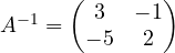 , as the 2×2 formula with
 confirms.
Why it works. Each elementary operation amounts to multiplying on the left by an elementary matrix  . If
 , then the product
 is exactly , and applied to it gives . If during the process a row on the left becomes all zeros, is not invertible.
A practical tip
To solve on a computer you never compute : it costs about three times as much as Gaussian elimination and is numerically less accurate. The inverse is a theoretical tool, useful for writing formulas; in programs you use  in MATLAB or numpy.linalg.solve.