Linear systems and Gaussian elimination
Matrix form, geometric meaning, elementary operations, row echelon form, inconsistent and underdetermined systems, Gauss-Jordan and the cost of the algorithm.
Solving a system of linear equations is the most common problem in applied mathematics: the currents in an electrical network, the forces in a truss, data interpolation, simulating a circuit in SPICE all come down to it. In this lesson we see how to write a system in matrix form, what it means geometrically and how to solve it with Gaussian elimination, which is also the algorithm computers use.
Linear systems and matrix form
A system of  linear equations in
 unknowns is written

where  is the coefficient matrix ( rows, columns),
 the vector of unknowns and
 the right-hand side. Placing next to gives the augmented matrix
 . If
 the system is homogeneous and always has at least the zero solution.
The geometric meaning
With two unknowns each equation is a line in the plane, and solving the system means finding the common points. There are only three possibilities.
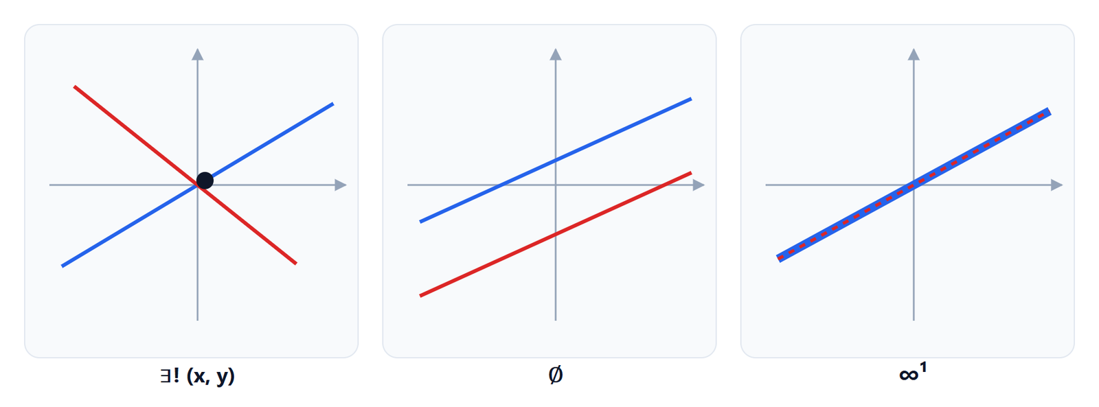
The same holds in general: a linear system has one solution, none or infinitely many. It cannot have exactly two, because if  and
 are solutions so is every point of the line through them,
 : indeed
 . With three unknowns each equation is a plane, and the solutions are a point, a line, a plane or nothing.
Elementary operations
The solutions of a system do not change if these elementary operations are applied to its equations (that is, to the rows of the augmented matrix):
- swap two rows;
- multiply a row by a non-zero number;
- add a multiple of one row to another row.
Each operation is invertible (it is undone by an operation of the same type), so every solution of the new system solves the old one and vice versa.
Gaussian elimination
The idea is to use elementary operations to bring the augmented matrix to row echelon form: each row starts with more zeros than the one above. The first non-zero entry of each row is called the pivot. Then the system is solved from the bottom up, by back substitution.
Example.
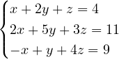

From the last row  , so
 . From the second
 . From the first
 . Solution:
 . It always pays to check it in the original third equation:
 . Correct.
Inconsistent and underdetermined systems
The echelon form tells you at once what is going on.
- If a row
 with
 appears, that is the equation
 , the system is inconsistent.
- Otherwise it can be solved. The unknowns matching the pivots are worked out; the others are free parameters. With unknowns and
 pivots the solutions depend on
 parameters.
Example.  ,
 ,
 . With
 and
 we get the rows
 and ; with
 the last becomes all zeros. Two pivots and three unknowns are left:
 free,
 ,
 . The solutions are the line
 .
Had the last row been  (for instance with 7 instead of 6 on the right of the third equation), the system would have been inconsistent: the three planes would have no common point.
Gauss-Jordan elimination
Carrying the elimination upwards as well and dividing each row by its pivot gives the reduced row echelon form: pivots equal to 1 and zeros above and below each pivot. The solutions can be read off directly, without substitution. The same procedure, applied to the matrix  , computes the inverse matrix (see the lesson on matrices).
How much it costs
For an  system elimination takes about
 operations. With
 that is just under a billion, a fraction of a second for a computer. Numerical libraries (LAPACK, used by MATLAB and NumPy) use exactly Gaussian elimination, in a form called LU factorisation, with partial pivoting: at each step the entry of largest absolute value in the column is chosen as pivot, so as not to divide by tiny numbers and to limit rounding errors.
A note for electronics people
With nodal analysis, each node of a linear circuit gives a linear equation in the node voltages (Kirchhoff’s current law). A circuit with 500 nodes is a  system, and a simulator such as SPICE, at every time step, does nothing but build it and solve it by Gaussian elimination, taking advantage of the fact that the matrix is almost entirely zeros.