Nodal analysis and mesh analysis
The node voltage method with an example, the matrix form, mesh analysis, dependent sources and checking the power balance.
Kirchhoff’s laws applied to every branch give a system of  equations: too many to write by hand even for a modest circuit. Systematic methods cut the unknowns drastically by choosing the right quantities: the node voltages (nodal analysis) or the mesh currents (mesh analysis). Nodal analysis in particular is the method used by SPICE and every circuit simulator.
Nodal analysis
- Choose a reference node (ground), at zero potential.
- The unknowns are the node voltages
 of the other nodes relative to the reference: there are
 of them.
- Write the current law at every node other than the reference, expressing each current through the node voltages: the current in a resistor between nodes
 and
 is
 .
- Solve the linear system.
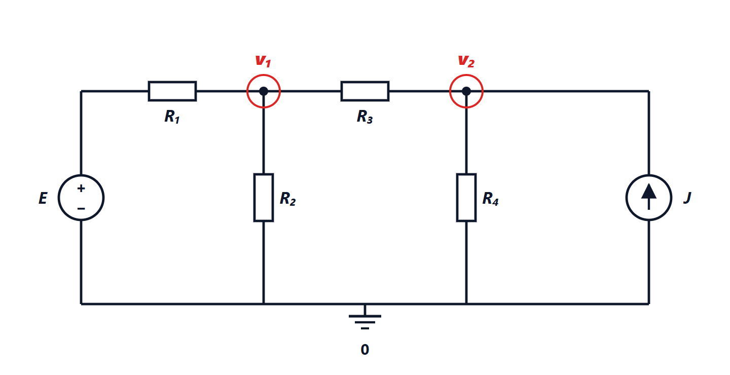
Example. In the circuit of the figure source  is connected between ground and the left end of
 . Current law at node 1 (outgoing currents positive):

and at node 2, where the current  enters:
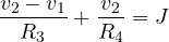
With  V,
 mA and all resistors 1 kΩ (currents in mA and voltages in V):

giving  V and
 V. Two equations instead of the twelve of the general method (6 branches).
Matrix form
With only resistors and current sources the system has a structure that can be written “by inspection”:

- on the diagonal,
 is the sum of the conductances connected to node
 ;
- off the diagonal,
 is minus the conductance between nodes and
 ;
 is the sum of the source currents entering node .
The matrix  is symmetric, diagonally dominant and sparse (each node connects to few others): the properties that make it fast to solve with the methods of the Numerical Analysis lesson on linear systems. Voltage sources are handled by turning them into current sources (if they have a series resistance) or by adding their current as an unknown: this is modified nodal analysis (MNA), used by SPICE.
Mesh analysis
It is the dual method, handy for planar circuits with many voltage sources.
- Assign to each “window” mesh (meshes that contain no others) a fictitious mesh current flowing round it.
- The current in a branch is the algebraic sum of the currents of the meshes it belongs to.
- Write the voltage law in each mesh.
There are  unknowns. Here too the matrix can be written by inspection: on the diagonal the sum of the mesh’s resistances, off the diagonal minus the shared resistances.
Which to choose. Count: nodal analysis has unknowns, mesh analysis . Choose the one with fewer, bearing in mind that current sources simplify nodal analysis and voltage sources mesh analysis.
Dependent sources
Many models of electronic components (transistors, operational amplifiers) contain controlled sources: their voltage or current depends on another quantity in the circuit. For example the small-signal model of a bipolar transistor contains a current source  , proportional to the base-emitter voltage. In nodal analysis they are treated like ordinary sources, then the controlling quantity is expressed through the node voltages: the matrix loses its symmetry, but the method stays the same.
An always useful check
After solving, it is worth checking the power balance: the total power delivered by the sources must equal the total power dissipated in the resistors. In the example: carries  mA, so delivers
 mW; delivers
 mW. The dissipated powers:
 mW, equal to the 60.6 mW delivered. It adds up.