The perceptron and multilayer networks: Novikoff's theorem, XOR and universal approximation
The perceptron and Novikoff's convergence theorem proved, the XOR problem, multilayer networks and activation functions, the universal approximation theorem, a 100-seed experiment on network size.
https://www.electronics-engineering.com/en/perceptron-multilayer-networks-xor-universal-approximation/
A neural network is a function built by composing many simple functions, the neurons: each computes a weighted sum of its inputs and passes it through a non-linear function. This lesson starts from the simplest neuron, Rosenblatt’s perceptron (1958), proves that it learns in a finite number of steps when the classes can be separated by a line, shows why a single layer is not enough (the XOR problem) and introduces multilayer networks, with the universal approximation theorem and an experiment showing how much the size of the network matters.
The perceptron
The perceptron classifies an input  into two classes,
 and
 , with the sign of a weighted sum:
 . Geometrically, the boundary between the classes is the hyperplane
 (a line in two dimensions). The learning algorithm is very simple: go through the examples and, when one is misclassified, move the weight vector towards it,

(the intercept  is included in
 by adding a constant component 1 to ).
Theorem (Novikoff, 1962). If there is a unit vector  that separates the data with margin
 , i.e.
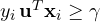 for every
 , and
 , the perceptron makes at most
 corrections.
Proof. Follow two quantities after  corrections, starting from
 . The projection on grows by at least
 at each correction:
 , so
 . The norm instead grows little:
 , because the correction happens only if
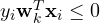 ; so
 . By the Cauchy-Schwarz inequality
 , i.e.
 . ∎
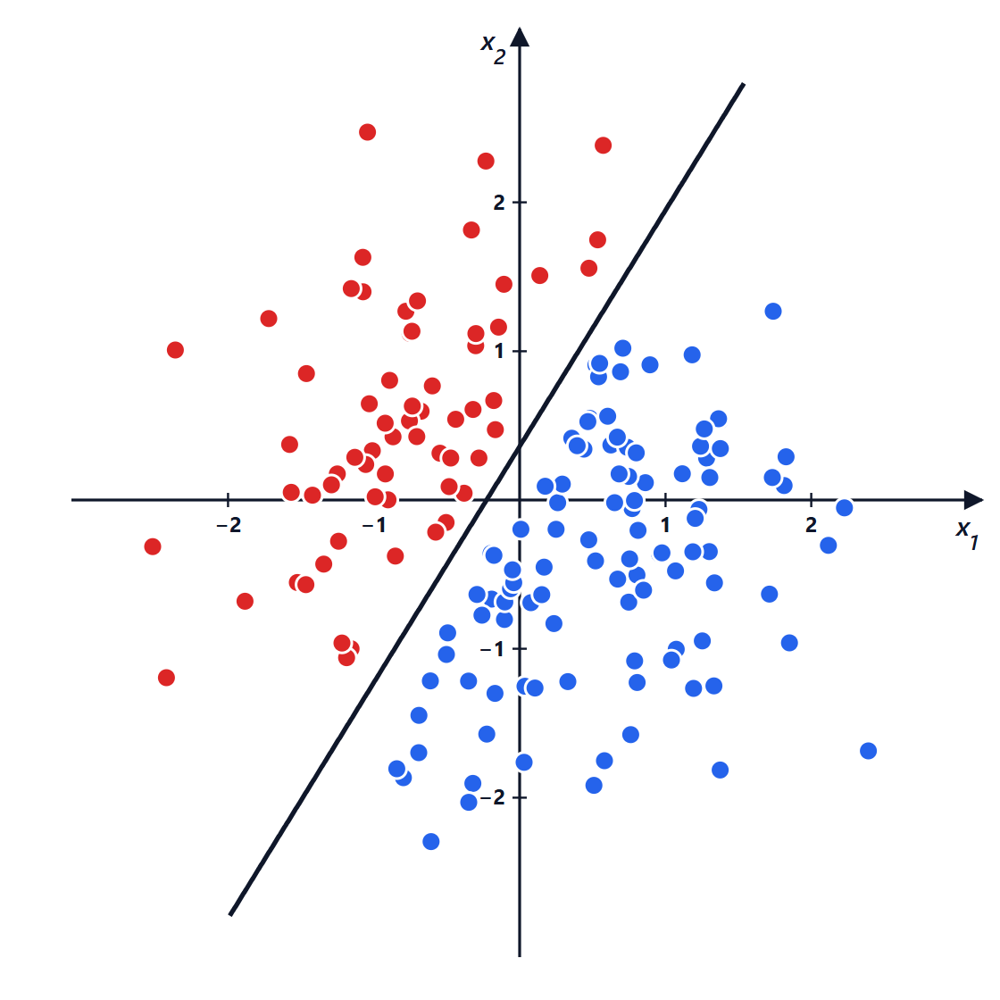
The bound depends neither on the number of examples nor on the dimension of the space, only on how “far apart” the classes are compared with their extent. In an experiment with 167 points separable with margin 0.15, the perceptron made 11 corrections in 3 passes over the data; Novikoff’s bound was 421: the theorem is a worst case, practice usually does much better.
The limit of one layer: XOR
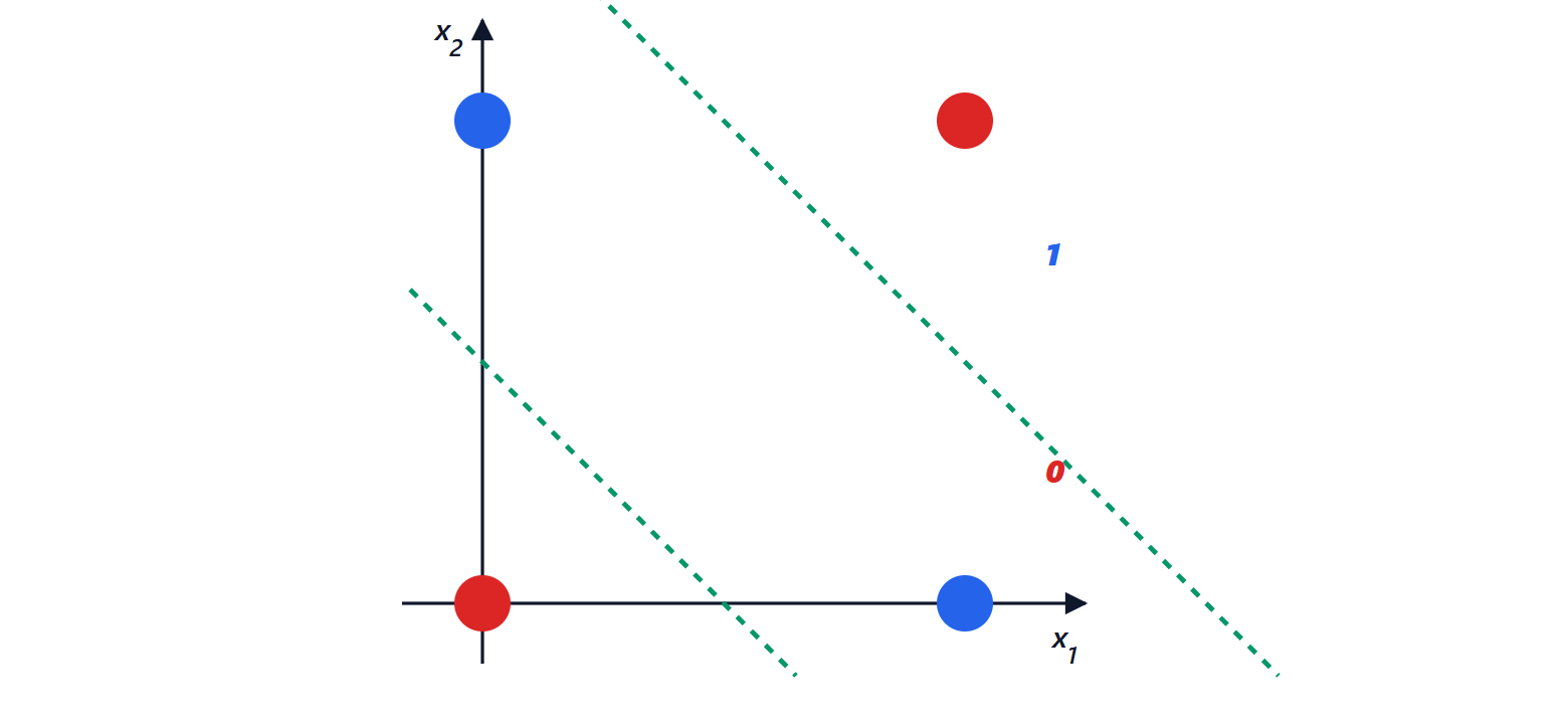
The perceptron finds a line, but many problems cannot be separated by a line. The simplest is XOR (exclusive or): the output is 1 if exactly one of the two inputs is 1. The points (0, 1) and (1, 0) must be on one side, (0, 0) and (1, 1) on the other: no line can do it. Minsky and Papert pointed this out in 1969, and research on neural networks slowed down for years.
The solution is to add a hidden layer: the hidden neurons turn the inputs into new variables in which the problem becomes separable. Two hidden neurons are enough: one can compute “at least one is 1” (OR), the other “both are 1” (AND), and the output “OR but not AND”.
Multilayer networks
A multilayer network (multilayer perceptron, MLP) applies linear transformations and non-linearities in sequence:

The activation function  is essential: without it, the composition of linear transformations is still linear and the network would be no more powerful than a single layer. The most used:
- sigmoid
 and hyperbolic tangent
 : smooth, but they “saturate” for large
 , where the derivative is almost zero;
- ReLU
 : very simple, derivative 1 for
 , does not saturate in one direction. It has been the default choice since 2012;
- smooth variants such as GELU and SiLU, used in transformers.
Universal approximation theorem (Cybenko 1989, Hornik 1991). A network with a single hidden layer and a non-polynomial activation can approximate with arbitrarily small error any continuous function on a closed and bounded set, provided it has enough neurons.
Proof idea (for one variable, with the sigmoid). A very steep sigmoid 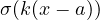 is almost a step at
 ; the difference of two steps is a “rectangle” between and
 . A continuous function can be approximated by a step function (sums of rectangles) with error as small as desired, by narrowing the steps; each rectangle costs two neurons. ∎
The theorem says the network can represent the function, not that gradient descent will find it, nor how many neurons are needed (they can be very many). In practice deep networks, with many layers of moderate width, represent useful functions with far fewer parameters than a wide shallow network: each layer builds more abstract features from those of the previous layer.
An experiment: how big must the network be
XOR is trained with gradient descent starting from random weights, repeating with 100 different seeds, and counting how many times the network really learns the function:
| hidden neurons | XOR solved |
|---|---|
| 2 | 49 times out of 100 |
| 3 | 92 times out of 100 |
| 4 | 98 times out of 100 |
With two hidden neurons the solution exists, but half of the time gradient descent stops in a local minimum (for example with output 0.5 on two of the four cases). Adding neurons, the error landscape becomes easier to travel and almost every starting point leads to a solution. It is one of the reasons why modern networks have many more parameters than would be needed in theory.
import numpy as np

X = np.array([[0, 0], [0, 1], [1, 0], [1, 1]], float)
y = np.array([0, 1, 1, 0], float)                          # XOR
sig = lambda z: 1 / (1 + np.exp(-z))

def train(hidden, seed, steps=10000, eta=0.5):
    g = np.random.default_rng(seed)
    W1, b1 = g.normal(0, 1, (2, hidden)), np.zeros(hidden)
    W2, b2 = g.normal(0, 1, hidden), 0.0
    for _ in range(steps):
        h = np.tanh(X @ W1 + b1)                           # hidden layer
        out = sig(h @ W2 + b2)
        d2 = out - y                                       # gradient of cross-entropy + sigmoid
        dh = np.outer(d2, W2) * (1 - h ** 2)               # derivative of tanh
        W2 -= eta * h.T @ d2; b2 -= eta * d2.sum()
        W1 -= eta * X.T @ dh; b1 -= eta * dh.sum(0)
    return sig(np.tanh(X @ W1 + b1) @ W2 + b2)

for hidden in (2, 3, 4):
    solved = sum(np.all(np.abs(train(hidden, s) - y) < 0.1) for s in range(100))
    print(f"{hidden} hidden neurons: XOR solved {solved} times out of 100")
print("example with 3 neurons:", np.round(train(3, 0), 3))
The gradient computation written by hand here, for one hidden layer, generalises to any number of layers with backpropagation, the subject of the next lesson.

Benvenuti nella pagina su «Il percettrone e le reti a più strati: teorema di Novikoff, XOR e approssimazione universale». L'ho scritta pensando a chi studia ingegneria elettronica: se un passaggio non vi torna, un esercizio vi dà un risultato diverso o volete altro materiale sull'argomento, chiedete pure nei commenti e vi risponderò. Un voto con le stelle qui sopra mi aiuta a capire quali pagine migliorare.Welcome to the page on “The perceptron and multilayer networks: Novikoff's theorem, XOR and universal approximation”. I wrote it for engineering students: if a step does not add up, an exercise gives you a different result or you would like more material on the topic, just ask in the comments and I will reply. A star rating above helps me understand which pages to improve.