Training in practice: data, He initialisation, normalisation, dropout and metrics

Between the theory of the previous lessons and a network that really works there are many practical choices: how to split the data, how to initialise the weights, how to normalise, how to avoid overfitting, how to measure the result. This lesson presents them with their mathematical reasons and with measured experiments, including those that do not confirm expectations: in network training many “tricks” work on some problems and not on others, and the only way to know is to measure.

Splitting the data

The data are split into three parts: training (for the weights), validation (for the choices: network size, step size, regularisation, when to stop) and test, used only once at the end to estimate performance on new data. If choices are made by looking at the test set, the test becomes a second validation and the estimate is optimistic. With little data cross-validation is used: the set is split into parts, training is done times leaving out a different one, and the results are averaged. Two practical warnings: the split must be done before any normalisation (mean and variance are computed on the training set only), and for data in time (sensor series) the test must come after the training data, not mixed in.

Weight initialisation

If the initial weights are too small the activations (and gradients) fade out layer after layer; if they are too large they explode. The right initialisation keeps the variance constant.

Theorem (He initialisation, 2015). In a network with ReLU activations, independent zero-mean weights and inputs per neuron, the variance of the weighted sums stays constant from one layer to the next if .

Proof. For a neuron with independent of and zero mean, . With and symmetric about zero, ReLU lets half of the distribution through: . So , which stays the same if . ∎

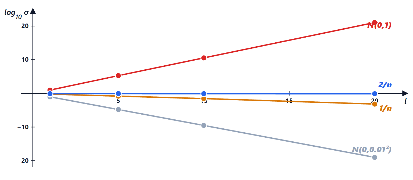
For symmetric activations such as tanh the factor 1/2 is absent and one gets (Xavier or Glorot, 2010). Experiment: 20 layers of 256 ReLU neurons, standard deviation of the activations:

weights	after 1 layer	after 5	after 10	after 20
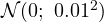	0.094
	9.35
Xavier,	0.58	0.15	0.028	0.00067
He,	0.83	0.86	0.80	0.76

With ReLU only He initialisation preserves the signal; Xavier’s halves it (in variance) at each layer, exactly the factor 1/2 of the proof.

Normalisation

Batch normalisation (2015) normalises the weighted sums of each neuron over the mini-batch (mean 0, variance 1) and then rescales them with two learned parameters. It makes training much less sensitive to initialisation and step size, and allows larger steps. In transformers layer normalisation is used, which normalises over the components of a single example instead of over the batch, and works even with small batches and sequences of variable length. The inputs too must be normalised: variables with very different scales (a temperature in kelvin and a voltage in millivolts) worsen the conditioning (lesson 1).

Against overfitting

• More data: the most effective remedy of all, as the experiment below shows.
• Data augmentation: new copies of the examples transformed in ways that do not change the answer (shifts, rotations, noise, lighting changes).
• Weight decay: the penalty of lesson 1.
• Dropout (Srivastava et al., 2014): during training each neuron is switched off at random with probability , and the remaining ones are multiplied by . In this way the expected value of each output is the same with and without dropout: , and in use the whole network is used without corrections. The idea is to prevent neurons from “leaning” on each other.
• Early stopping: the validation error is monitored during training and training stops when it starts to rise.

The experiments. Dense network 64 → 1024 → 1024 → 10 on the 8×8 digits, trained for 300 steps on subsets of increasing size, accuracy on the 450 test digits (average over 3 seeds):

Dropout (p = 0.5), on the same network with 100 examples, gave 89.5 % against 89.1 % without (average over 5 seeds): no measurable difference; with 50 examples 77.8 % against 77.9 %. Weight decay with made it slightly worse (86.0 %). On this problem, small and already easy, regularisation matters little and the amount of data matters a lot. On very large networks and harder problems (ImageNet images, language models) dropout and weight decay instead give measurable benefits. The moral is the lesson’s: techniques must be tried on your own problem, with honest validation.

Metrics

Accuracy (fraction of right answers) is misleading when classes are unbalanced: if a fault happens in 1 % of cases, a classifier that always says “no fault” has 99 % accuracy and is useless. For a “positive” class, with TP, FP, FN the true positives, false positives and false negatives:

Precision says how many of the alarms are true, recall how many of the true cases are found. Moving the decision threshold trades one for the other; which matters more depends on the application (in an emergency braking system a false negative is much more serious than a false positive, in a spam filter the opposite). The confusion matrix, used in the last lesson, shows all errors class by class.

Choosing hyperparameters

Step size, sizes, regularisation, batch size are hyperparameters: they are not learned by the gradient, they are chosen by comparing results on the validation set. Random search (Bergstra and Bengio, 2012) is usually better than grid search: if only a few hyperparameters really matter, trying random values explores many more different values of the important ones. The step size is searched on a logarithmic scale (, , , …).

import numpy as np, torch, torch.nn as nn
from sklearn.datasets import load_digits
from sklearn.model_selection import train_test_split

# 1) initialisation: standard deviation of the activations through 20 ReLU layers
g = np.random.default_rng(0)
h0 = g.normal(0, 1, (1000, 256))
for name, std in (("N(0, 0.01^2)", lambda n: 0.01), ("N(0, 1)", lambda n: 1.0),
                  ("Xavier 1/n", lambda n: np.sqrt(1 / n)), ("He 2/n", lambda n: np.sqrt(2 / n))):
    h, values = h0.copy(), []
    for layer in range(20):
        h = np.maximum(h @ g.normal(0, std(256), (256, 256)), 0)
        values.append(h.std())
    print(f"{name:13s}: after 1, 5, 10, 20 layers {values[0]:.3g}, {values[4]:.3g}, {values[9]:.3g}, {values[19]:.3g}")

# 2) amount of data: the same network trained on larger and larger subsets
d = load_digits()
Xa, Xp, ya, yp = train_test_split(d.data / 16.0, d.target, test_size=0.25, random_state=0, stratify=d.target)
Xa, Xp = torch.tensor(Xa, dtype=torch.float32), torch.tensor(Xp, dtype=torch.float32)
ya, yp = torch.tensor(ya), torch.tensor(yp)

def trial(n, seed, dropout=0.0):
    torch.manual_seed(seed)
    layers = [nn.Linear(64, 1024), nn.ReLU()] + ([nn.Dropout(dropout)] if dropout else []) \
           + [nn.Linear(1024, 1024), nn.ReLU()] + ([nn.Dropout(dropout)] if dropout else []) + [nn.Linear(1024, 10)]
    net = nn.Sequential(*layers)
    opt = torch.optim.Adam(net.parameters(), lr=1e-3)
    idx = torch.randperm(len(Xa), generator=torch.Generator().manual_seed(seed))[:n]
    for _ in range(300):                                   # 300 steps on the whole subset
        net.train()
        loss = nn.functional.cross_entropy(net(Xa[idx]), ya[idx])
        opt.zero_grad(); loss.backward(); opt.step()
    net.eval()                                             # dropout is off in use
    with torch.no_grad():
        return float((net(Xp).argmax(1) == yp).float().mean())

for n in (50, 100, 200, 400, 1347):
    print(f"{n:4d} examples: test accuracy {np.mean([trial(n, s) for s in range(3)]):.3f}")