Project: recognising handwritten digits in NumPy and PyTorch, up to ONNX and 8-bit quantisation
A network written from scratch in NumPy and the same one in PyTorch on 8x8 digits (98 % accuracy), confusion matrix and error analysis, ONNX export and 8-bit weight quantisation for microcontrollers.
This lesson puts the whole course together in a complete, working project: recognising handwritten digits. The network is first written from scratch in NumPy, with the backpropagation of lesson 3, then the same network in PyTorch, where the gradients are computed by automatic differentiation; the result is evaluated with the confusion matrix and the errors are examined; finally the model is prepared for use outside Python (ONNX format) and for a microcontroller, with 8-bit weight quantisation. All the numbers reported come from running the code at the bottom of the page.
The data
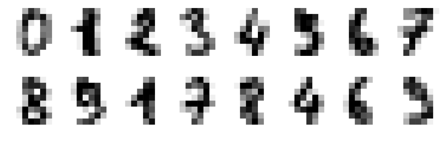
The scikit-learn collection contains 1797 digits handwritten by 43 people, reduced to 8×8 pixel images with 17 grey levels (from 0 to 16): small enough to train a network in a second on a laptop, but a real problem, with different handwriting. The values are divided by 16 (inputs between 0 and 1, lesson 7) and the data are split into 1347 training examples and 450 test examples, stratified (each digit in the same proportion in the two sets) and with a fixed seed, so that the result is reproducible.
The network in NumPy
Architecture 64 → 64 → 10: 64 inputs (the pixels), one hidden layer of 64 ReLU neurons, 10 outputs with softmax. Weights initialised with He’s rule (lesson 7), cross-entropy, stochastic gradient descent with batches of 32 examples and step 0.1 for 100 epochs. The training loop is the direct translation of the backpropagation equations:  , last-layer gradients
 ,
 , first-layer gradients
 . Result: 98.0 % test accuracy, in 0.3-0.4 seconds.
The same network in PyTorch
In PyTorch the network is declared as a sequence of layers, and the gradient is computed by loss.backward(). With the same architecture, the same optimiser and the same hyperparameters one gets 97.8 %: the small difference (one example out of 450) comes from the different random initialisation (PyTorch uses a scaled uniform distribution by default) and from the batch order. For such a small network PyTorch is even slower than NumPy (1.6 s): the real advantage comes with large networks, on the GPU, and with complicated architectures whose derivatives nobody would want to write by hand.
The confusion matrix
Rows: true digit; columns: digit predicted by the PyTorch network. On the diagonal the right answers:
| 0 | 1 | 2 | 3 | 4 | 5 | 6 | 7 | 8 | 9 | |
|---|---|---|---|---|---|---|---|---|---|---|
| 0 | 45 | |||||||||
| 1 | 45 | 1 | ||||||||
| 2 | 1 | 43 | ||||||||
| 3 | 46 | |||||||||
| 4 | 1 | 43 | 1 | |||||||
| 5 | 1 | 1 | 44 | |||||||
| 6 | 1 | 44 | ||||||||
| 7 | 45 | |||||||||
| 8 | 2 | 41 | ||||||||
| 9 | 1 | 44 |
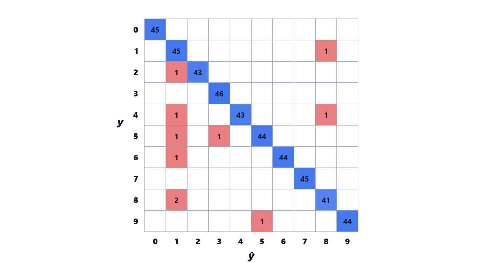
Ten errors out of 450, and half end up in the column of 1: at 8×8 pixels a slightly thick vertical stroke is enough to make an 8, a 4 or a 6 look like a 1. Looking at where a model goes wrong is the most useful step to improve it: here it would suggest higher-resolution images, a CNN (lesson 5), or more examples of the confused pairs.
From model to product
- Saving:
torch.savesaves the weights; to reload them the same network code is needed. - ONNX (Open Neural Network Exchange):
torch.onnx.exportsaves network and weights in a standard format, which runs with ONNX Runtime in C++, C#, Java or JavaScript, on servers, phones or in the browser, without Python. - Microcontrollers: a network can also run on a microcontroller with a few hundred kilobytes of memory (TensorFlow Lite for Microcontrollers, or C code generated by tools such as STM32Cube.AI). The decisive step is quantisation: weights become 8-bit integers,
 with
 between −127 and 127 and one scale
 per matrix. Weight memory shrinks fourfold and computations become integer operations, much faster and cheaper in energy. On the digit network weight memory drops from 18,944 to 4,736 bytes and accuracy does not change (97.8 %). On larger networks the loss is usually a few tenths of a point; when it is too much, the network is trained taking quantisation into account (quantisation-aware training).
The complete code
import time
import numpy as np
from sklearn.datasets import load_digits
from sklearn.model_selection import train_test_split

# data: 1797 handwritten digits, 8x8 pixels with values 0..16
d = load_digits()
Xtr, Xte, ytr, yte = train_test_split(d.data / 16.0, d.target, test_size=0.25, random_state=0, stratify=d.target)

# ---------------- network from scratch in NumPy: 64 -> 64 (ReLU) -> 10 (softmax) ----------------
rng = np.random.default_rng(0)
W1 = rng.normal(0, np.sqrt(2 / 64), (64, 64)); b1 = np.zeros(64)       # He initialisation
W2 = rng.normal(0, np.sqrt(2 / 64), (64, 10)); b2 = np.zeros(10)

def forward(X):
    z1 = X @ W1 + b1
    h = np.maximum(z1, 0)
    z2 = h @ W2 + b2
    p = np.exp(z2 - z2.max(1, keepdims=True))
    return h, p / p.sum(1, keepdims=True)

t0 = time.time()
LR, EPOCHS, BATCH = 0.1, 100, 32
for epoch in range(EPOCHS):
    perm = rng.permutation(len(Xtr))
    for i in range(0, len(Xtr), BATCH):
        idx = perm[i:i + BATCH]
        X, y = Xtr[idx], ytr[idx]
        h, p = forward(X)
        d2 = p.copy(); d2[np.arange(len(y)), y] -= 1; d2 /= len(y)    # gradient of softmax + cross-entropy
        gW2, gb2 = h.T @ d2, d2.sum(0)
        d1 = (d2 @ W2.T) * (h > 0)                                    # backpropagation through the ReLU
        gW1, gb1 = X.T @ d1, d1.sum(0)
        W1 -= LR * gW1; b1 -= LR * gb1; W2 -= LR * gW2; b2 -= LR * gb2
acc_np = (forward(Xte)[1].argmax(1) == yte).mean()
print(f"NumPy: test accuracy {acc_np:.4f} in {time.time() - t0:.1f} s")

# ---------------- the same network in PyTorch ----------------
import torch
import torch.nn as nn

torch.manual_seed(0)
model = nn.Sequential(nn.Linear(64, 64), nn.ReLU(), nn.Linear(64, 10))
opt = torch.optim.SGD(model.parameters(), lr=LR)
Xt, yt = torch.tensor(Xtr, dtype=torch.float32), torch.tensor(ytr)
t0 = time.time()
for epoch in range(EPOCHS):
    perm = torch.randperm(len(Xt))
    for i in range(0, len(Xt), BATCH):
        idx = perm[i:i + BATCH]
        loss = nn.functional.cross_entropy(model(Xt[idx]), yt[idx])  # autograd computes the gradient
        opt.zero_grad(); loss.backward(); opt.step()
with torch.no_grad():
    pred = model(torch.tensor(Xte, dtype=torch.float32)).argmax(1).numpy()
print(f"PyTorch: test accuracy {(pred == yte).mean():.4f} in {time.time() - t0:.1f} s")

# confusion matrix: rows = true digit, columns = predicted digit
conf = np.zeros((10, 10), int)
for t, q in zip(yte, pred):
    conf[t, q] += 1
print(conf)

# 8-bit weight quantisation (symmetric, one scale per matrix), as on microcontrollers
qmodel = nn.Sequential(nn.Linear(64, 64), nn.ReLU(), nn.Linear(64, 10))
qmodel.load_state_dict(model.state_dict())
with torch.no_grad():
    for layer in (qmodel[0], qmodel[2]):
        scale = layer.weight.abs().max() / 127                         # the largest weight becomes 127
        q = torch.round(layer.weight / scale).clamp(-127, 127)          # integers from -127 to 127
        layer.weight.copy_(q * scale)                                   # values the network actually sees
    qpred = qmodel(torch.tensor(Xte, dtype=torch.float32)).argmax(1).numpy()
print(f"8-bit weights: test accuracy {(qpred == yte).mean():.4f}, weight memory {sum(p.numel() for p in model.parameters() if p.dim() == 2)} bytes instead of {4 * sum(p.numel() for p in model.parameters() if p.dim() == 2)}")
torch.save(model.state_dict(), "digits.pt")
torch.onnx.export(model, torch.zeros(1, 64), "digits.onnx")                 # to use it outside Python
What comes next
The course has built all the pieces: gradient descent, multilayer networks, backpropagation, optimisers, convolutions, sequences and attention, training practice. The same ideas, scaled up by many orders of magnitude, are those of vision models and language models. The reinforcement learning course shows how networks learn to decide instead of recognise, with an environment in place of labelled data.