Convolutional networks: convolution, translation equivariance, pooling and sizes
Two-dimensional convolution, translation equivariance proved, pooling, size and parameter-count formulas, LeNet, AlexNet and ResNet, dense network versus CNN on handwritten digits.
A one-megapixel colour image has three million values: a dense network with a thousand neurons in the first layer would have three billion weights there alone, and would have to learn separately that a cat at the top left and a cat at the bottom right are the same thing. Convolutional networks (CNNs) solve both problems with two ideas taken from signal processing: the weights are local (each neuron looks only at a small area) and shared (the same filter slides over the whole image). This lesson defines convolution, proves the property that makes CNNs suited to images (translation equivariance), derives the size formulas, and compares a CNN with a dense network on handwritten digits.
Convolution
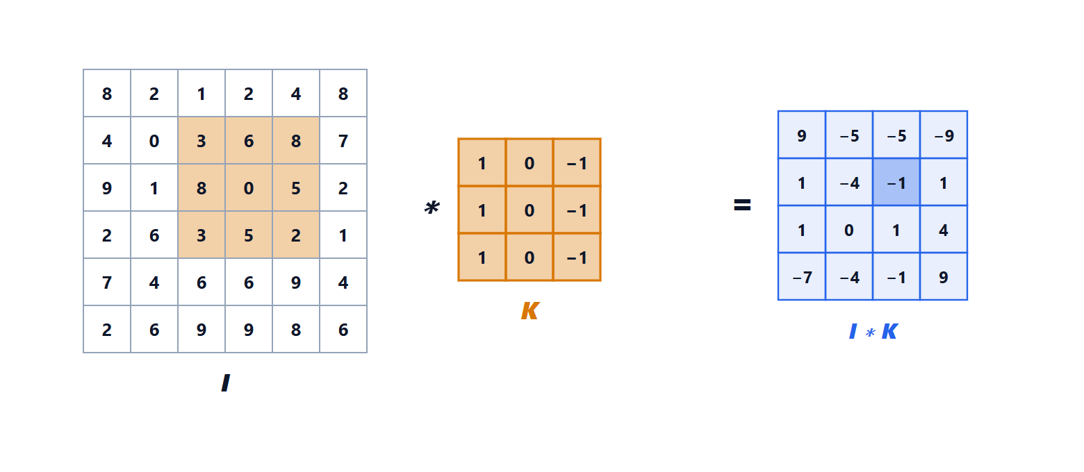
A convolutional layer applies a small filter (kernel)  , for example 3×3, at every position of the image
 :

(neural networks use this form, which strictly speaking is a correlation; true convolution has the filter flipped, but since the filter is learned the difference does not matter). It is the same FIR filter of digital signal processing, in two dimensions. With several input channels (the three colours, or the outputs of the previous layer) the filter has one channel for each and the contributions are summed; with several filters several output feature maps are obtained.
A 3×3 filter with values  on every row, for example, responds to vertical edges. The network is not given hand-written filters: it learns them with backpropagation, and in the first layers of a trained CNN edge and colour-blob detectors appear; in the following layers, increasingly complex combinations (corners, textures, object parts).
Why it works: translation equivariance
Theorem. Convolution commutes with translations: if the image is shifted, the output map shifts by the same amount. With  the translation
 :
 .
Proof.  . ∎
An eye detector learned in a corner of the image automatically works everywhere: it need not be learned again for every position. This inductive bias (prior knowledge about the problem, built into the network’s structure) greatly reduces the parameters and data needed. To also obtain partial invariance (same response even if the object moves) pooling is added: 2×2 max-pooling replaces each 2×2 block of values with the maximum, halving the size and making the network insensitive to small shifts.
Sizes
For an input of side  , filter of side
 , padding
 (border of zeros added) and stride
 , the output side is

(the filter starts at position 0 and can make  moves). With
 ,
 ,
 the output has the same size as the input. A layer with
 input channels and
 filters has
 parameters, independently of the image size. The receptive field (the input area influencing a neuron) grows by
 pixels for every 3×3 layer and doubles with every pooling: stacking layers, deep neurons “see” the whole image.
Historical architectures show the evolution: LeNet (1998) read postcodes; AlexNet (2012) won the ImageNet competition by a huge margin using GPUs and ReLU, starting the deep learning era; ResNet (2015) added residual connections  , which let the gradient cross hundreds of layers without vanishing.
The experiment: dense network versus convolutional network
On scikit-learn’s 1797 8×8 handwritten digits (1347 for training, 450 for testing), two networks trained with Adam for 60 epochs:
- dense network: 64 inputs → 64 ReLU neurons → 10 outputs;
- CNN: two 3×3 convolutional layers (8 and 16 filters) with ReLU, a 2×2 max-pooling, a final dense layer.
| network | parameters | test accuracy | with the image shifted by 1 pixel |
|---|---|---|---|
| dense | 4,810 | 96.9 % | 42.9 % |
| convolutional | 3,818 | 98.2 % | 65.1 % |
The CNN is more accurate with fewer parameters, because the convolutional structure already tells it that neighbouring pixels must be looked at together. Shifting all test images one pixel to the right (a minimal change for a human eye), the dense network collapses to 43 %: it has learned “this pixel lit means 7”, not the shape. The CNN holds up better but still loses a lot, because on 8×8 images one pixel is more than 10 % of the width and pooling gives only a little invariance. In practice data augmentation is added: training also on shifted, rotated, scaled copies of the images.
import numpy as np, torch, torch.nn as nn
from sklearn.datasets import load_digits
from sklearn.model_selection import train_test_split

d = load_digits()
Xa, Xp, ya, yp = train_test_split(d.data / 16.0, d.target, test_size=0.25, random_state=0, stratify=d.target)
Xa, Xp = torch.tensor(Xa, dtype=torch.float32), torch.tensor(Xp, dtype=torch.float32)
ya, yp = torch.tensor(ya), torch.tensor(yp)

def train(model, epochs=60):
    torch.manual_seed(0)
    opt = torch.optim.Adam(model.parameters(), lr=1e-3)
    for _ in range(epochs):
        perm = torch.randperm(len(Xa))
        for i in range(0, len(Xa), 64):
            idx = perm[i:i + 64]
            loss = nn.functional.cross_entropy(model(Xa[idx]), ya[idx])
            opt.zero_grad(); loss.backward(); opt.step()
    return model

def accuracy(model, X):
    with torch.no_grad():
        return float((model(X).argmax(1) == yp).float().mean())

torch.manual_seed(0)
dense = nn.Sequential(nn.Linear(64, 64), nn.ReLU(), nn.Linear(64, 10))
torch.manual_seed(0)
cnn = nn.Sequential(nn.Unflatten(1, (1, 8, 8)),                    # from 64 values to a 1x8x8 image
                    nn.Conv2d(1, 8, 3, padding=1), nn.ReLU(),       # 8 filters 3x3
                    nn.Conv2d(8, 16, 3, padding=1), nn.ReLU(),      # 16 filters 3x3x8
                    nn.MaxPool2d(2),                                # 8x8 -> 4x4
                    nn.Flatten(), nn.Linear(16 * 4 * 4, 10))
train(dense); train(cnn)

shifted = torch.roll(Xp.view(-1, 8, 8), 1, dims=2)                  # all digits one pixel to the right
shifted[:, :, 0] = 0
shifted = shifted.view(-1, 64)
for name, m in (("dense", dense), ("convolutional", cnn)):
    n = sum(p.numel() for p in m.parameters())
    print(f"{name:15s}: {n} parameters, test {accuracy(m, Xp):.4f}, shifted {accuracy(m, shifted):.4f}")