Backpropagation: equations proved in matrix form and numerical gradient check

To train a network with gradient descent the derivative of the loss with respect to every weight is needed: millions, or billions, of derivatives at each step. Computing them one by one would be impossible. Backpropagation (popularised by Rumelhart, Hinton and Williams in 1986) computes them all at a cost of the same order as evaluating the network (about three times in total), applying the chain rule backwards, from the output towards the input. This lesson derives it in matrix form for a multilayer network, explains why it is so efficient, implements it from scratch in NumPy and checks it with the numerical gradient check.

The computational graph and the chain rule

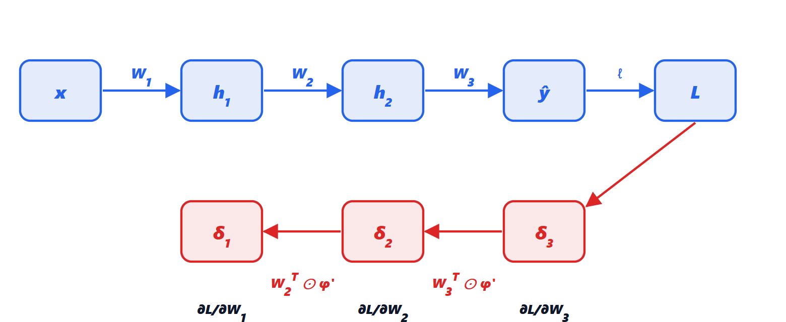
A network is a composition of functions: . By the chain rule, the derivative with respect to a parameter of an inner layer is the product of the derivatives of all the layers that follow it. The key observation is that these products have common factors: the derivative with respect to the output of layer is needed for the parameters of layer and also, multiplied by one more factor, for all previous layers. Computing it only once, starting from the end, avoids repeating work. It is the same principle as dynamic programming.

Backpropagation for a multilayer network

For a network with layers , (with ), the layer error is defined as .

Theorem (the backpropagation equations).

where is the element-wise product.

Proof. Component of depends on through . By the chain rule , which in vector form is the second equation. For the weights: , so and . ∎

The last layer. With softmax and cross-entropy (lesson 1), : the predicted probability minus the true one (encoded “one-hot”, 1 in the right class and 0 elsewhere). With a mini-batch of examples, and become matrices with one example per row, and the formulas become (averaged over the batch): matrix products, exactly what GPUs are very fast at.

The cost. The forward pass costs one matrix-vector product per layer; the backward pass two (one for , one for the weight gradient). In total about three times the forward pass alone, regardless of the number of parameters. Computing derivatives with finite differences would instead require one forward pass for every parameter.

Automatic differentiation

Modern libraries (PyTorch, JAX, TensorFlow) do not ask you to write these formulas. During the forward pass they record every operation in a computational graph; calling backward() they traverse it backwards applying to each operation its known derivative. This is reverse-mode automatic differentiation: backpropagation generalised to any program, including conditions and loops. It is not a numerical approximation: the derivatives are exact, up to rounding.

The numerical gradient check

When backpropagation (or a new layer) is written by hand, it is checked with central differences: for a weight , , with an error of order (the odd orders of the Taylor expansion cancel). With and double-precision computations, a correct implementation gives a relative error around –; even a small mistake in the formula gives values of order or more.

import numpy as np

def initialise(sizes, seed=0):
    g = np.random.default_rng(seed)
    return [(g.normal(0, np.sqrt(2 / a), (a, b)), np.zeros(b)) for a, b in zip(sizes[:-1], sizes[1:])]

def forward(params, X):
    activations = [X]
    for i, (W, b) in enumerate(params):
        z = activations[-1] @ W + b
        activations.append(np.maximum(z, 0) if i < len(params) - 1 else z)     # ReLU, last layer linear
    return activations

def loss_and_gradients(params, X, Y):
    act = forward(params, X)
    z = act[-1] - act[-1].max(1, keepdims=True)
    p = np.exp(z); p /= p.sum(1, keepdims=True)                                 # softmax
    N = len(X)
    loss = -np.log(p[np.arange(N), Y]).mean()                                   # cross-entropy
    delta = p.copy(); delta[np.arange(N), Y] -= 1; delta /= N                   # delta of the last layer: p - y
    gradients = []
    for i in range(len(params) - 1, -1, -1):
        W, b = params[i]
        gradients.append((act[i].T @ delta, delta.sum(0)))                      # dL/dW = h^T delta
        if i > 0:
            delta = (delta @ W.T) * (act[i] > 0)                                # delta backwards, ReLU derivative
    return loss, gradients[::-1]

rng = np.random.default_rng(1)
X = rng.normal(0, 1, (8, 5)); Y = rng.integers(0, 3, 8)                         # 8 examples, 5 inputs, 3 classes
par = initialise([5, 7, 3])
_, grad = loss_and_gradients(par, X, Y)

eps, numerical = 1e-6, np.zeros_like(par[0][0])
for i in range(5):
    for j in range(7):
        par[0][0][i, j] += eps;     Lp, _ = loss_and_gradients(par, X, Y)
        par[0][0][i, j] -= 2 * eps; Lm, _ = loss_and_gradients(par, X, Y)
        par[0][0][i, j] += eps
        numerical[i, j] = (Lp - Lm) / (2 * eps)                                 # central differences
error = np.abs(numerical - grad[0][0]).max() / np.abs(numerical).max()
print(f"relative error between backpropagation and central differences: {error:.1e}")

Running it gives a relative error of about –: backpropagation is correct. The same two functions, with a gradient descent loop, are enough to train a real network: it is the project of the last lesson of the course, which recognises handwritten digits with 98 % accuracy.