Sequences: recurrent networks, vanishing gradient, LSTM, attention and transformers

Texts, audio signals, sensor time series, trajectories: many data are sequences, in which order matters and length varies. This lesson presents the two families of networks for sequences. Recurrent networks (RNNs) read one element at a time and carry a state with them; it is proved why their gradient vanishes on long sequences and how LSTMs avoid this. Transformers (2017) look at the whole sequence together with the attention mechanism; it is proved why the dot product must be divided by . Transformers are today the basis of language models and are increasingly used for images and signals too.

Recurrent networks

An RNN updates a hidden state at each element of the sequence, with the same weights at every step:

It is a non-linear discrete-time dynamical system, like those of Systems Theory, with learned parameters. To train it the network is “unrolled” in time (one copy per step) and backpropagation is applied: this is backpropagation through time (BPTT).

Theorem (vanishing or exploding gradient). , so .

Proof. By the chain rule 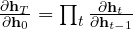, and differentiating with gives . The norm of a product is at most the product of the norms, and . ∎

If the gradient decreases exponentially with distance: the network cannot learn that an input far in the past determines today’s output. If it is greater than 1 it can explode (it is limited by clipping the gradient norm, as in PPO).

The LSTM

The LSTM (long short-term memory, Hochreiter and Schmidhuber, 1997) adds a memory cell controlled by three gates (values between 0 and 1 given by sigmoids):

The forget gate decides how much of the memory to keep, the input gate how much to write into it, the output gate how much of it to show. The key point is that the cell is updated by addition: , with no multiplications by or derivatives of saturating functions. If the network learns , the gradient crosses many steps almost intact. The GRU (2014) is a simpler variant with two gates.

The measurement. For freshly initialised networks (32-neuron state, average over 10 initialisations) automatic differentiation computes how much the output at the last step depends on the first input:

length	RNN	LSTM
1
10
20
50
100

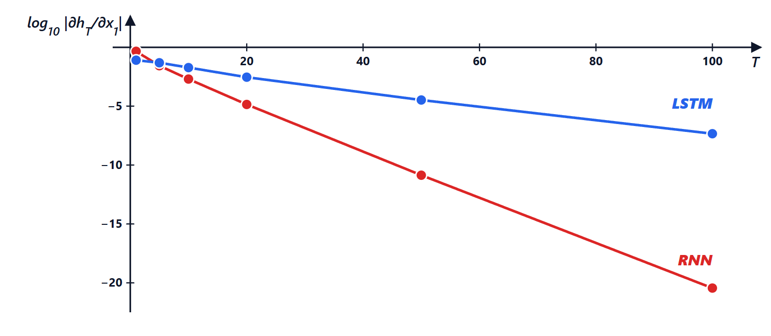
In the RNN the signal shrinks by a factor of about 0.6 at each step (the straight line on a logarithmic scale); after 100 steps it is times weaker than in the LSTM.

Attention

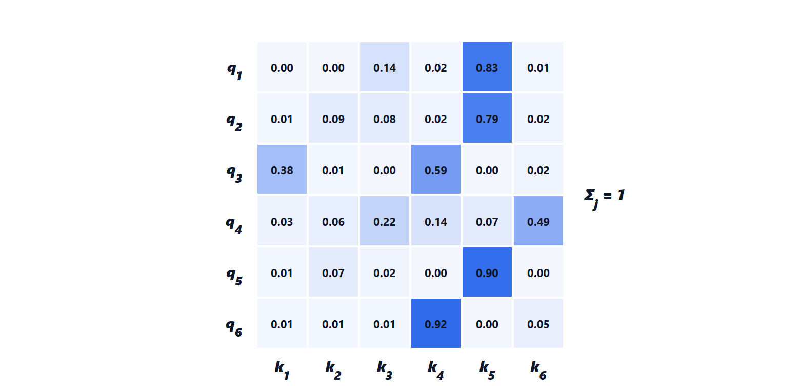
Even the LSTM struggles beyond a few hundred steps, and above all it works sequentially: step waits for step , and it cannot be parallelised on the GPU. Attention directly connects every position with all the others. Each element produces three vectors: a query , a key and a value , with learned weight matrices. The output for a position is an average of the values of all positions, weighted by how much its query “resembles” each key:

where the rows of are the queries, keys and values of the positions, and is the key dimension.

Theorem (why divide by ). If the components of and are independent with mean 0 and variance 1, the dot product has mean 0 and variance .

Proof. . Each term has mean and variance ; the terms are independent, so the variances add: . ∎

With the scores would have a standard deviation of about 23: the softmax of such large numbers is almost “one only, all the others zero”, and its gradient is almost zero. Dividing by brings the variance back to 1. In simulation (code at the end): variance 4.0, 64.0 and 509 for , and 1.00, 1.00, 0.99 after the division.

The transformer

The transformer (Vaswani et al., 2017, “Attention is all you need”) stacks identical blocks, each with:

• multi-head attention: several attentions in parallel, with different matrices, which can specialise (one follows syntax, another references);
• a small dense network applied to each position separately;
• residual connections and normalisation (layer norm) around both, as in ResNets.

Attention knows nothing about order (permuting the positions permutes the outputs in the same way), so a positional encoding is added to the inputs: in the original work sinusoids of different frequencies, today often rotations (RoPE). The cost of attention grows as with the sequence length , and it is the main limit of long-context models. In exchange all positions are computed in parallel, and this, more than anything else, is what made it possible to train models with hundreds of billions of parameters. To generate text a causal mask is used: each position can only look at the previous ones, and the model learns to predict the next word.

The code

import numpy as np
import torch, torch.nn as nn

# 1) attention in NumPy
def attention(Q, K, V):
    scores = Q @ K.T / np.sqrt(K.shape[1])
    weights = np.exp(scores - scores.max(1, keepdims=True))
    weights /= weights.sum(1, keepdims=True)               # row-wise softmax
    return weights @ V, weights

g = np.random.default_rng(0)
X = g.normal(0, 1, (6, 16))                                # 6 positions, 16 dimensions
Wq, Wk, Wv = (g.normal(0, 0.25, (16, 8)) for _ in range(3))
output, weights = attention(X @ Wq, X @ Wk, X @ Wv)
print("output", output.shape, "- the weight rows sum to", np.round(weights.sum(1), 6))

# 2) variance of the dot product before and after dividing by sqrt(d_k)
for dk in (4, 64, 512):
    q, k = g.normal(0, 1, (20000, dk)), g.normal(0, 1, (20000, dk))
    s = (q * k).sum(1)
    print(f"d_k = {dk:3d}: variance {s.var():6.1f}, after division {(s / np.sqrt(dk)).var():.3f}")

# 3) sensitivity of the last output to the first input, freshly initialised RNN versus LSTM
def sensitivity(kind, T, H=32, inits=10):
    values = []
    for s in range(inits):
        torch.manual_seed(s)
        net = (nn.RNN if kind == "rnn" else nn.LSTM)(1, H, batch_first=True)
        if kind == "lstm":                                 # forget gate initially open (bias 1)
            for name, p in net.named_parameters():
                if "bias_ih" in name:
                    p.data[H:2 * H] = 1.0
        x = torch.randn(1, T, 1, requires_grad=True)
        outputs, _ = net(x)
        outputs[0, -1].sum().backward()
        values.append(x.grad[0, 0].abs().item())
    return sum(values) / len(values)

for T in (1, 10, 20, 50, 100):
    print(f"T = {T:3d}: RNN {sensitivity('rnn', T):.1e}, LSTM {sensitivity('lstm', T):.1e}")