Vehicle dynamics in depth: bicycle model proved, Pacejka, load transfer, ABS, ESC, ACC, LKA and pure pursuit in Python
Full derivation of the bicycle model, proofs of steady-state steering and stability, Pacejka's magic formula with B, C, D, E, friction circle, relaxation length, load transfer, ABS, ESC, ACC, LKA and pure pursuit, with verified Python simulations.
This page takes the vehicle dynamics lesson to the level of detail needed by those who work on ADAS functions and stability control. It derives the bicycle model step by step, proves the stability conditions and the understeer formulas, describes the tyre with Pacejka’s model (the coefficients B, C, D, E and their meaning), the friction ellipse and the relaxation length, computes load transfers, and shows how these models become the ESC, ABS, ACC, LKA controllers and pure pursuit path tracking. The simulations are in Python, with verified code.
Numerical values of an average car used in the examples:  kg,
 kg·m²,
 m,
 m (
 m),
 kN/rad and
 kN/rad (cornering stiffness of each axle), centre of gravity height
 m.
The bicycle model, derived
Kinematics. In the vehicle-fixed frame (x forwards, y to the left) the centre of gravity has velocity  and the vehicle rotates with yaw rate
 . A point at distance
 ahead of the centre of gravity along
 has velocity
 (rigid motion:
 ). So the centre of the front axle (
 ) has lateral velocity
 and the rear one (
 )
 .
Slip angles. The angle between the wheel direction and the direction of its centre is, for the front wheel steered by  ,
 , and for the rear
 . With small angles and constant
 they linearise:
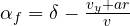 ,
 .
Dynamics. The frame rotates with the vehicle: the derivative of velocity in a rotating frame contains the term  , whose lateral component is
 . Newton’s second law along
 and the moment equation about
 give, with the axle lateral forces
 and
 (the front force is almost perpendicular to the vehicle axis for small ):

Substituting the slip angles gives the state form  with
 :

The lateral acceleration measured by an accelerometer at the centre of gravity is  .
Steady state, understeer and stability, proved
Theorem (steady-state steering). In a steady turn of radius  , with
 and
 :

Proof. In steady state  . From the moment equation
 ; from Newton’s
 . So
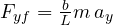 and
 : each axle carries the fraction of centripetal force corresponding to the load it supports. The slip angles are
 ,
 . Subtracting the kinematic expressions:
 . Hence
 . ∎
The sign of  tells which axle “slips more”: if the front slips more than the rear the vehicle understeers. With the example data
 mrad/(m/s²)
 ° per m/s²: in a bend at 4 m/s² (0.4 g) 0.77° more road-wheel steering than geometry is needed, about 12° at the steering wheel with a steering ratio of 15.
Theorem (stability). The bicycle model is stable at every speed if  ; if
 it becomes unstable above
 .
Proof. A  system is stable if and only if the trace of
 is negative and the determinant positive. The trace is always negative. Computing the determinant and simplifying with
 :

(using  ). With it is always positive; with it vanishes at
 and beyond becomes negative: a real pole moves into the right half-plane. ∎
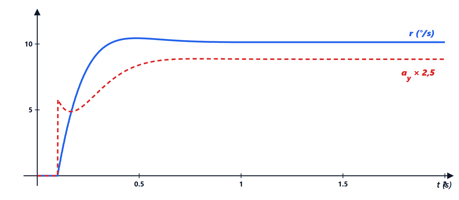
The transfer function steering → yaw rate has static gain 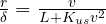 and poles that move with speed. With the example data (computed with the code below): at 10 m/s
 rad/s and
 ; at 20 m/s 9.1 rad/s and 0.84; at 30 m/s 7.2 rad/s and 0.70. The vehicle becomes slower and less damped as speed increases: this is what the driver feels as a “lazier, more swaying” response on the motorway.
The tyre: Pacejka’s model
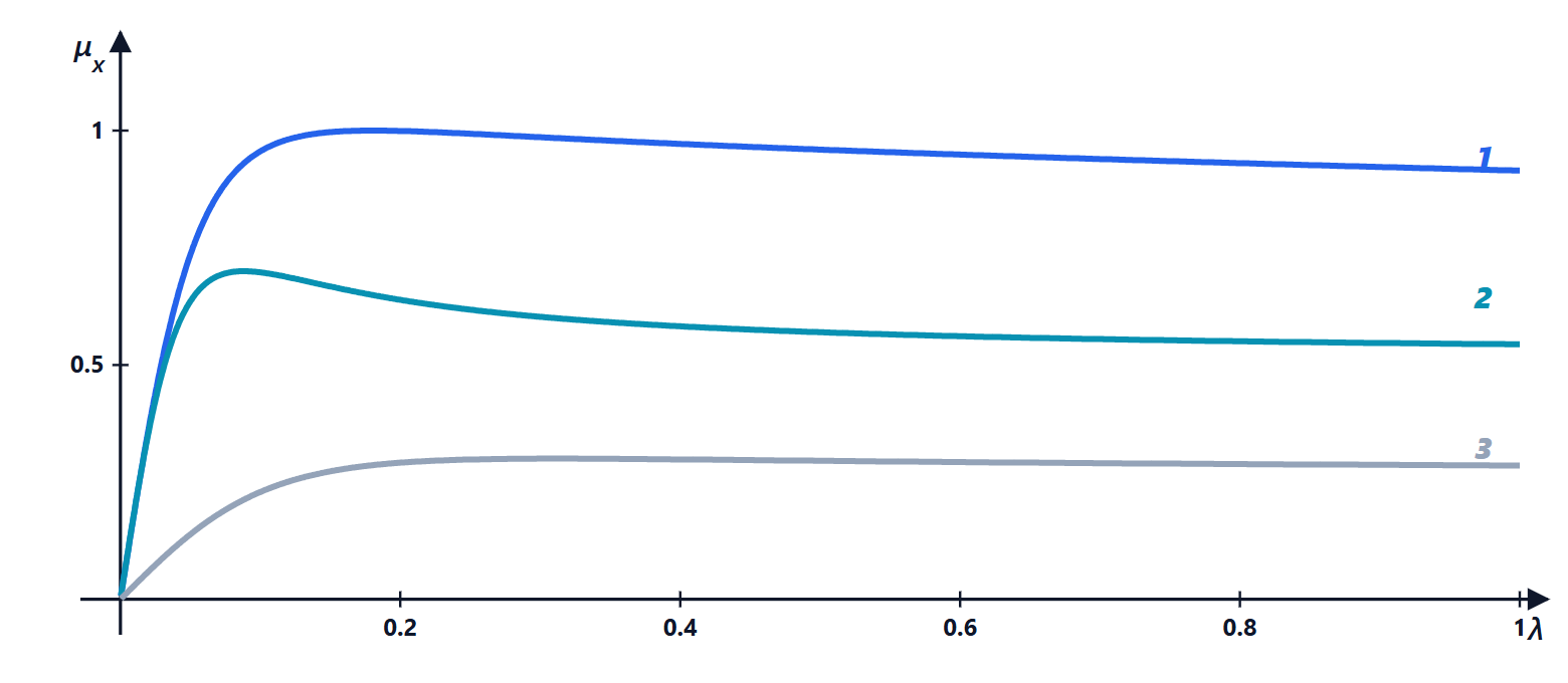
Pacejka’s magic formula describes measured forces with a few constants:

with the slip angle (for the lateral force) or the slip ratio (for the longitudinal one), and
 the peak value, about
 ;
 the shape factor, which decides how much the curve drops after the peak (about 1.3 for lateral force, 1.6-1.9 for longitudinal);
 the stiffness factor: the slope at the origin is
 , i.e. the cornering stiffness
 ;
 the curvature, which shapes the curve near the peak.
In complete models (MF 5.2, MF 6.1, used in industry simulators) each coefficient in turn depends on load, camber and pressure through dozens of parameters measured on a test rig. Two effects matter even in simple models:
- load sensitivity:
 and
 grow less than proportionally with
 . This is why two wheels with different loads give less total lateral force than two wheels with the same average load: lateral load transfer “takes away” grip from the axle where it is larger;
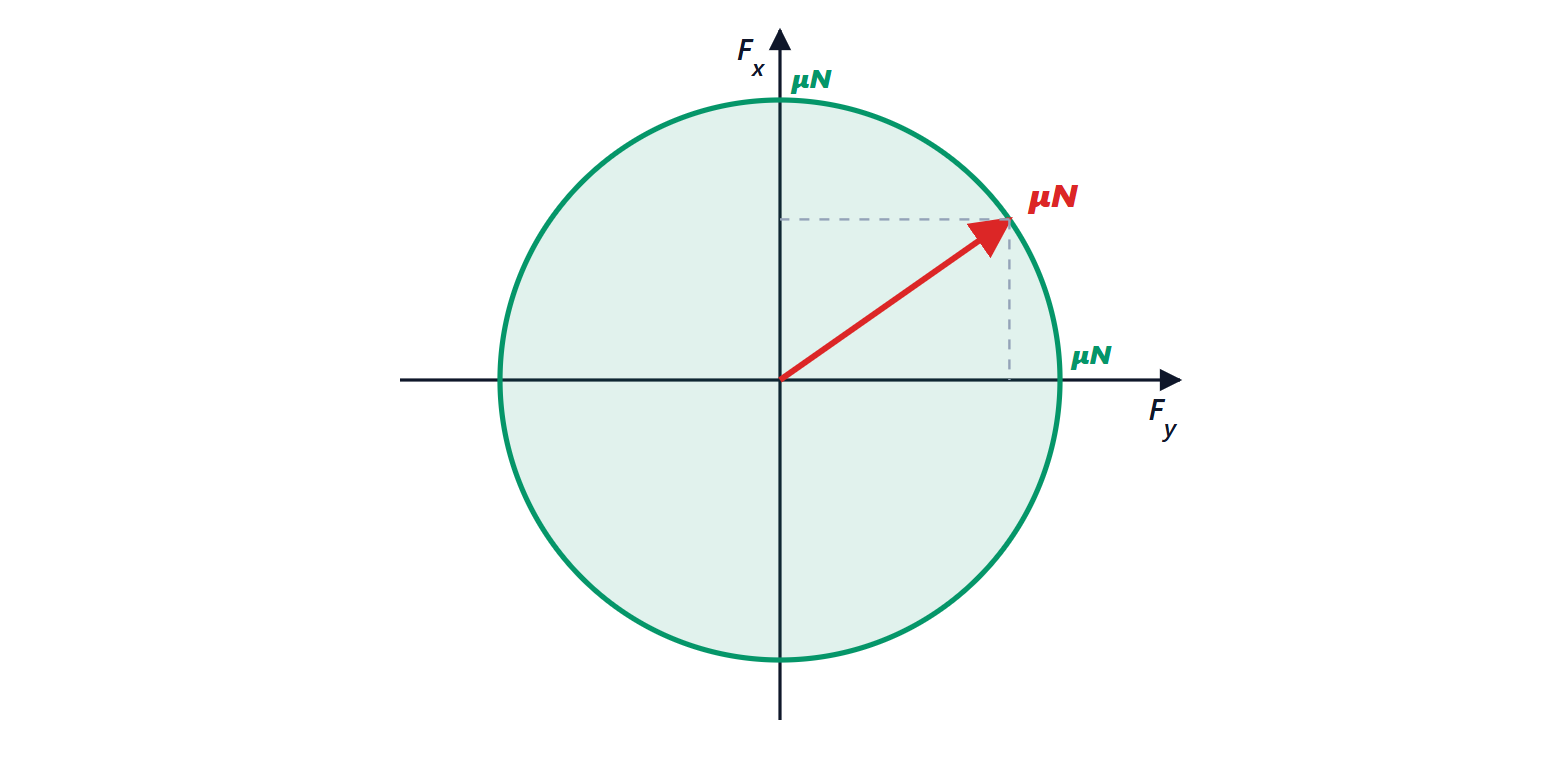
- friction ellipse: the total force cannot exceed about , in any direction:
 . Braking in a bend takes away lateral force: this is why ABS leaves the steered wheels able to generate force.
Relaxation length. The tyre does not generate force instantly: it has to roll a distance  (of the order of 0.3-0.5 m) for the deformation to settle. The model is a first-order lag
 , with time constant
 : at low speed the tyre is “slow”, and this matters in stability control at 10-20 km/h.
Load transfers
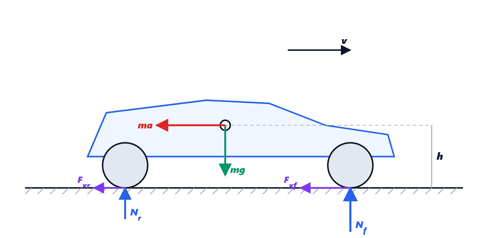
Longitudinal. When braking with deceleration  , moment balance about the rear contact point, with the inertial force
 applied at the centre of gravity at height
 , gives

With the example data and  : at rest 8.49 kN front and 6.23 rear; when braking 10.98 and 3.74 kN. This is why front brakes are larger and brake distribution must adapt to load (electronic brake-force distribution EBD): locking the rear wheels first makes the vehicle unstable.
Lateral. In a bend, on each axle of track  , load moves from the inner to the outer wheel by
 , with a split between the axles decided by the anti-roll bar stiffnesses. Because of load sensitivity, the axle with more transfer loses more cornering stiffness: stiffening the front bar makes the vehicle more understeering, stiffening the rear one more oversteering. It is the most used adjustment on the track.
From the wheel to ABS
The dynamics of a wheel is  , with
 the torque (drive or brake) and
 . When braking, if the brake torque exceeds what the road can return at the peak of
 , the wheel decelerates faster and faster and locks (
 ): the tyre slides, loses lateral grip and the vehicle no longer steers. ABS estimates slip from the wheel speeds and modulates brake pressure to keep it near the peak (about 0.1-0.2), with 5-15 cycles per second. Traction control does the same when accelerating by reducing engine torque or braking the spinning wheel.
ESC: stability control
ESC compares the measured yaw rate with a reference given by the bicycle model and limited by grip:

The limit comes from  . If exceeds the reference the vehicle oversteers: the outer front wheel is braked, creating a straightening moment. If is too small the vehicle understeers: the inner rear wheel is braked. The controller is typically a PI on the yaw error with activation logic, and it works together with ABS on the same brakes.
The kinematic model and pure pursuit
At low speed slip is negligible: wheels move where they point. The kinematic bicycle model, referred to the rear axle, is

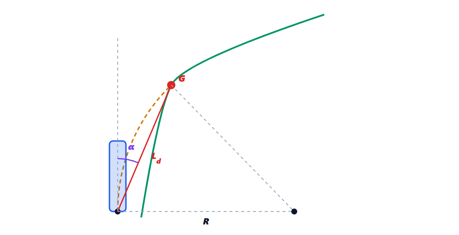
Theorem (pure pursuit). To reach, along a circular arc, a point  of the path at distance
 and seen at an angle
 from the vehicle axis, the curvature
 is needed, i.e. the steering
 .
Proof. The required circle is tangent to the vehicle axis at the rear axle and passes through . Its centre lies on the perpendicular to the axis, at distance . The triangle formed by the centre, the rear axle and is isosceles (two sides are radii), and the angle at the centre is  (the angle between chord and tangent is half the central angle). So
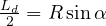 ,
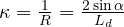 . In the kinematic model
 , giving . ∎
is the only parameter: small gives precise but oscillating tracking, large gives smooth tracking that “cuts” corners. It is usually increased with speed,  .
ACC and LKA
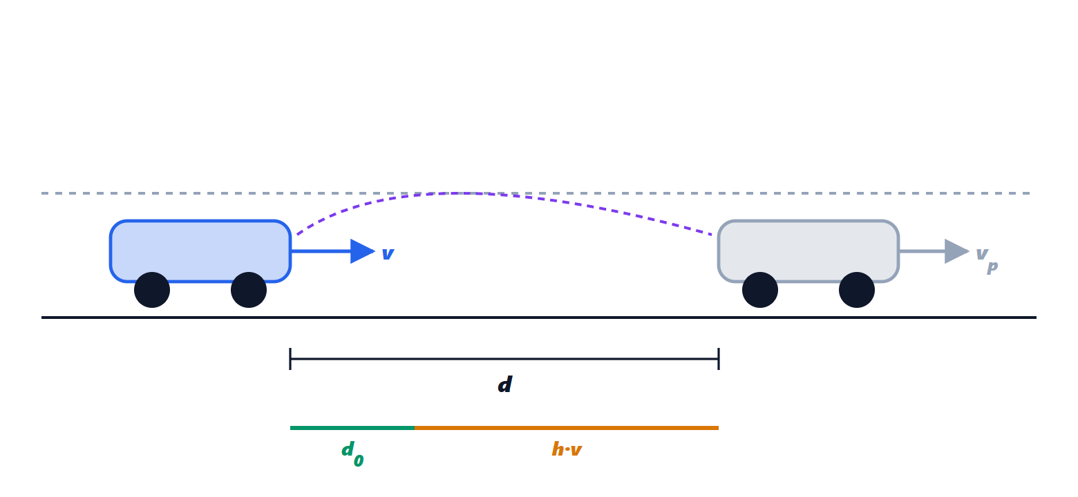
ACC. With the distance  from the preceding vehicle and its speed
 , the constant time-gap policy wants
 . A simple controller commands an acceleration
 , then limited for comfort (about −3 to +2 m/s²) and implemented by the engine and brake torque control. In a platoon of vehicles all with ACC, the time-gap policy with large enough guarantees string stability: a disturbance of the first vehicle is not amplified along the line.
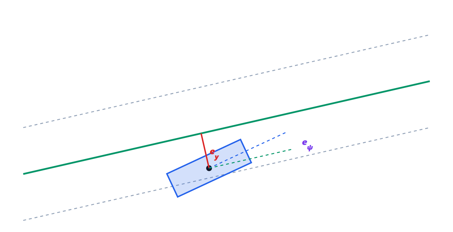
LKA. The bicycle model is written relative to the lane:  the lateral offset from the centre,
 the angle between the vehicle and the lane tangent,
 the road curvature. For small angles
 and
 : with the state
 a fourth-order linear model is obtained (Rajamani) on which a state-feedback (LQR) or predictive (MPC) controller is designed, with the curvature as a measured disturbance to be compensated in advance.
Simulations in Python
The bicycle model, with gains and poles at various speeds and the step response:
import numpy as np

# parameters of an average car
m, Iz = 1500.0, 2500.0        # mass [kg], yaw moment of inertia [kg m^2]
a, b = 1.1, 1.5               # distances of the CG from the front and rear axle [m]
L = a + b                     # wheelbase [m]
Cf, Cr = 100e3, 120e3         # axle cornering stiffnesses [N/rad]

def matrices(v):
    """Linear bicycle model: state x = [vy, r], input delta (road-wheel steering)."""
    A = np.array([[-(Cf + Cr) / (m * v), -v - (a * Cf - b * Cr) / (m * v)],
                  [-(a * Cf - b * Cr) / (Iz * v), -(a**2 * Cf + b**2 * Cr) / (Iz * v)]])
    B = np.array([Cf / m, a * Cf / Iz])
    return A, B

Kus = m / L * (b / Cf - a / Cr)               # understeer gradient [rad/(m/s^2)]
vch = np.sqrt(L / Kus)                         # characteristic speed [m/s]
print(f"Kus = {Kus*1e3:.2f} mrad/(m/s^2) = {np.degrees(Kus):.3f} deg/(m/s^2)")
print(f"characteristic speed = {vch:.1f} m/s = {vch*3.6:.0f} km/h")

for v in (10.0, 20.0, 30.0):
    A, B = matrices(v)
    x_ss = -np.linalg.solve(A, B)              # steady state for delta = 1 rad
    lam = np.linalg.eigvals(A)
    wn = np.sqrt(np.prod(lam).real); zeta = -lam.real.sum() / (2 * wn)
    print(f"v = {v:4.1f} m/s: r/delta = {x_ss[1]:.3f} 1/s (formula {v/(L + Kus*v**2):.3f}), "
          f"poles {np.round(lam, 2)}, wn = {wn:.2f} rad/s, zeta = {zeta:.2f}")

# response to a 2 degree steering step at 20 m/s (Euler, 1 ms step)
v, dt = 20.0, 0.001
A, B = matrices(v)
x = np.zeros(2); d = np.radians(2.0)
t_hist, r_hist, ay_hist = [], [], []
for k in range(3000):
    dx = A @ x + B * d
    ay = dx[0] + v * x[1]                      # lateral acceleration
    x = x + dt * dx
    t_hist.append(k * dt); r_hist.append(x[1]); ay_hist.append(ay)
r = np.array(r_hist)
print(f"2 deg step at 20 m/s: final r {np.degrees(r[-1]):.2f} deg/s, "
      f"final ay {ay_hist[-1]:.2f} m/s^2, peak r {np.degrees(r.max()):.2f} deg/s")
Running it prints mrad/(m/s²), characteristic speed 27.8 m/s (100 km/h), the gains 3.405, 5.068 and 5.330 s equal to the formula, the poles and damping ratios quoted above, and for the step
 °/s,
 m/s² with a peak of 10.44°/s.
Pure pursuit on a 3.5 m lane change at 10 m/s:
import numpy as np

L, v, dt = 2.6, 10.0, 0.01            # wheelbase [m], speed [m/s], integration step [s]
Ld = 8.0                               # look-ahead distance [m]
delta_max = np.radians(30)

# reference path: smooth 3.5 m lane change (sinusoid)
xs = np.linspace(0, 200, 4001)
ys = np.where(xs < 50, 0.0, np.where(xs > 90, 3.5, 1.75 * (1 - np.cos(np.pi * (xs - 50) / 40))))

x, y, psi = 0.0, 0.0, 0.0              # rear-axle position and heading
err = []
for k in range(int(15 / dt)):
    # path point at distance Ld ahead of the vehicle
    d = np.hypot(xs - x, ys - y)
    ahead = np.where((d >= Ld) & (xs > x))[0]
    gx, gy = xs[ahead[0]], ys[ahead[0]]
    alpha = np.arctan2(gy - y, gx - x) - psi            # angle towards point G
    delta = np.arctan(2 * L * np.sin(alpha) / Ld)        # pure pursuit law
    delta = np.clip(delta, -delta_max, delta_max)
    # kinematic bicycle model (referred to the rear axle)
    x += v * np.cos(psi) * dt
    y += v * np.sin(psi) * dt
    psi += v / L * np.tan(delta) * dt
    err.append(y - np.interp(x, xs, ys))
err = np.array(err)
print(f"max lateral error {abs(err).max():.2f} m, final {abs(err[-1]):.3f} m")
The maximum lateral error is 7 cm and at the end it vanishes. For more complete models industry uses commercial simulators (IPG CarMaker, VI-grade, CarSim, MATLAB’s Vehicle Dynamics Blockset); in the open world there are CARLA (autonomous driving, with a Python API) and the Modelica vehicle models, usable with OpenModelica.
The exercises on understeer, tyres, load transfer, braking and ADAS functions are on the exercise page linked at the top.