Regression and gradient descent: normal equations, convergence, logistic regression and overfitting
The supervised learning problem, the normal equations proved, convergence of gradient descent with the 2/L limit, logistic regression and cross-entropy, overfitting and ridge regularisation with experiments.
https://www.electronics-engineering.com/en/linear-regression-gradient-descent-overfitting/
Machine learning builds models that learn from data instead of being programmed rule by rule: one chooses a family of functions with parameters, defines an error measuring how far predictions are from the data, and looks for the parameters that minimise it. All neural networks, even the largest, work this way. This first lesson presents the ingredients with the simplest models: linear regression (with the exact solution and the iterative one of gradient descent, whose convergence is proved), logistic regression for classification, and the central problem of the whole course, overfitting.
The supervised learning problem
There are  examples
 : an input (a sensor’s measurements, an image’s pixels) and the right answer (a temperature, a digit). We want a function
 that predicts
 also for new inputs. A loss
 is chosen and its average over the data is minimised:

The real goal however is not to do well on the data at hand, but on the data that will come: this is why some examples are set aside (validation set and test set), not used for training and only used to measure.
Linear regression and the normal equations
With  (adding a constant component 1 to
 , the first weight acts as the intercept) and the squared error, putting the examples in the rows of a matrix
 :
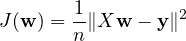
Theorem. If  is invertible, the minimum is
 (normal equations).
Proof.  is a convex quadratic function; the gradient is
 and vanishes for
 . The Hessian
 is positive definite (if the columns of are independent), so the stationary point is the only minimum. Geometrically,
 is the orthogonal projection of
 onto the space spanned by the columns of : the residual
 is perpendicular to all columns. ∎
Gradient descent
For more complicated models there is no closed formula. One starts from any  and takes small steps in the direction in which the error decreases fastest, the opposite of the gradient:

with  the learning rate. It is the algorithm that trains all neural networks.
Theorem (convergence on a quadratic). For a quadratic with positive definite Hessian  , with eigenvalues
 , gradient descent converges to
 from any starting point if and only if
 .
Proof. For a quadratic  , so the error
 evolves as
 . In the eigenvectors of each component is multiplied at every step by
 , and tends to zero if and only if
 , i.e.
 . The strictest condition is that of the largest eigenvalue,
 . ∎
The speed depends on the condition number  : with the best step the reduction factor per step is
 , close to 1 when the eigenvalues are very different. This is why inputs are normalised (same scale for all variables) and why the optimisers of lesson 4 exist.
Numerical example. With 50 points  noise, the normal equations give
 . For these data
 : gradient descent with
 ,
 and
 converges to the same result (with
 213 steps are needed for an error of
 ), while with
 , just beyond the limit, it diverges to values of
 .
Classification: logistic regression
To predict a class (yes or no, fault or no fault) the sigmoid  is used, which turns any number into a probability:
 .
Theorem. Maximising the likelihood of the data is equivalent to minimising the cross-entropy  , with
 , and the gradient is
 .
Proof. The probability of observing  is
 ; for independent examples the likelihood is the product, and its logarithm with changed sign and divided by is . For the gradient one uses
 :
 . ∎
The gradient has the same form as in linear regression: (prediction − truth) × input. With several classes the sigmoid becomes the softmax  and the gradient with respect to
 is still
 : it is the last layer of almost all classification networks.
Overfitting
A model that is too flexible also learns the noise in the data. With 15 points of  plus noise, polynomials of increasing degree are fitted and the mean squared error is measured on the training data and on 200 new points:
| degree | training error | error on new data |
|---|---|---|
| 1 | 0.252 | 0.259 |
| 3 | 0.013 | 0.095 |
| 9 | 0.007 | 0.808 |
| 14 | 0.002 | 50.2 |
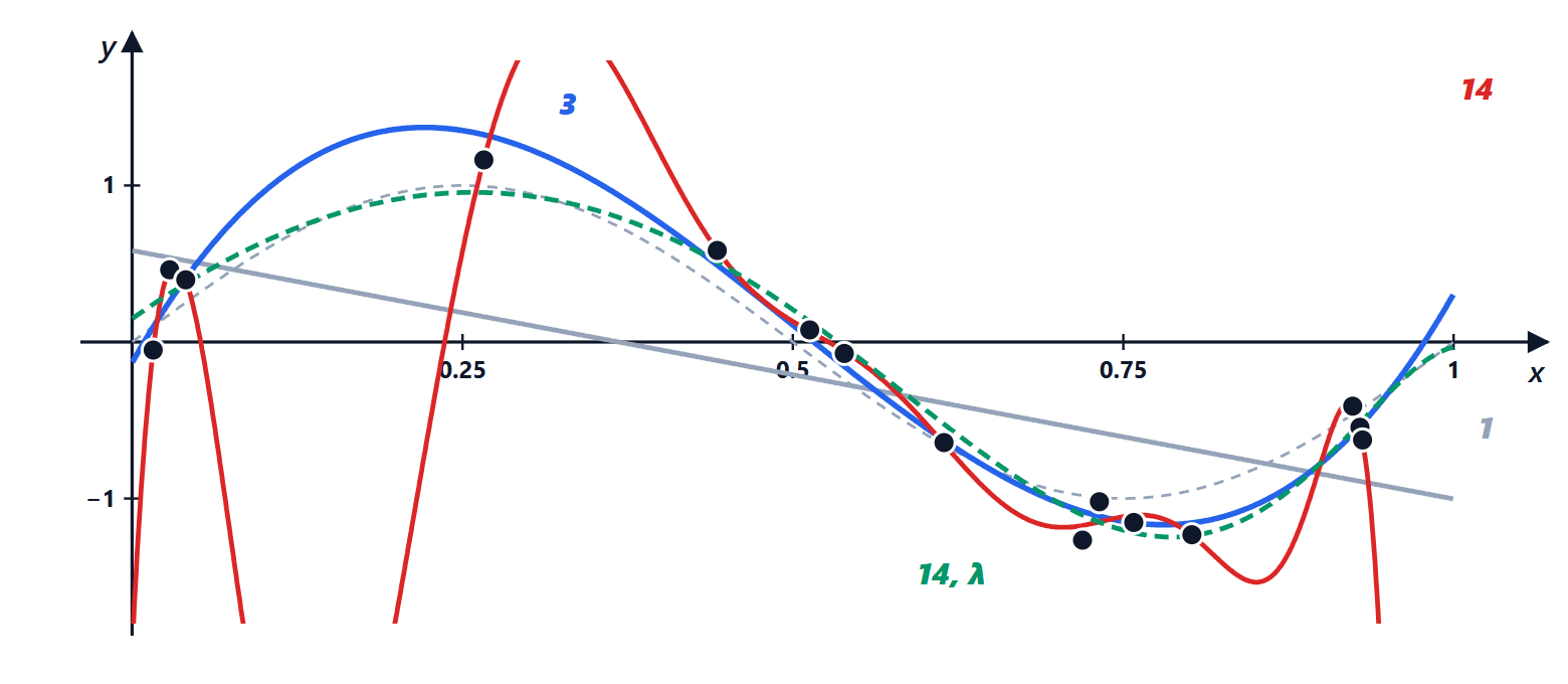
The training error always decreases, the error on new data first decreases and then explodes. Degree 1 underfits (too simple: high bias), degree 14 overfits (too flexible: high variance). This is the bias-variance trade-off: the expected error on a new point decomposes into squared bias, plus the model’s variance as the data change, plus irreducible noise.
Regularisation penalises large weights:  (ridge, or weight decay in networks), with solution
 (same proof as the normal equations). On the degree-14 polynomial with
 the error on new data drops from 50.2 to 0.069, better even than degree 3. The value of
 is chosen by looking at the validation set, never at the test set.
The code
import numpy as np

rng = np.random.default_rng(0)
x = rng.uniform(0, 1, 50)
y = 2 + 3 * x + rng.normal(0, 0.3, 50)
X = np.c_[np.ones(50), x]                                   # column of 1s for the intercept

w_exact = np.linalg.solve(X.T @ X, X.T @ y)                 # normal equations
L = 2 * np.linalg.eigvalsh(X.T @ X / 50).max()              # largest eigenvalue of the Hessian
print("normal equations:", np.round(w_exact, 4), " step limit 2/L =", round(2 / L, 3))
for eta in (0.5, 0.9 * 2 / L, 1.1 * 2 / L):
    w = np.zeros(2)
    for k in range(2000):
        w -= eta * 2 / 50 * X.T @ (X @ w - y)              # gradient descent
    print(f"eta = {eta:.3f}:", np.round(w, 4) if np.all(np.isfinite(w)) else "diverges")

# overfitting: polynomials on 15 points, error on 200 new points
f = lambda t: np.sin(2 * np.pi * t)
xa = np.sort(rng.uniform(0, 1, 15)); ya = f(xa) + rng.normal(0, 0.2, 15)
xn = rng.uniform(0, 1, 200); yn = f(xn) + rng.normal(0, 0.2, 200)
def fit(degree, lam=0.0):
    A = np.vander(xa, degree + 1, increasing=True)
    return np.linalg.solve(A.T @ A + lam * np.eye(degree + 1), A.T @ ya)      # ridge if lam > 0
def error(c, xs, ys):
    return np.mean((np.vander(xs, len(c), increasing=True) @ c - ys) ** 2)
for degree, lam in ((1, 0), (3, 0), (9, 0), (14, 0), (14, 1e-3)):
    c = fit(degree, lam)
    print(f"degree {degree:2d}, lambda {lam:g}: training {error(c, xa, ya):.4f}, new data {error(c, xn, yn):.4f}")
Running it reproduces the numbers in the text. The following lessons replace the linear model with neural networks, which are still trained by gradient descent and suffer from the same overfitting problems.





Benvenuti nella pagina su «Regressione e discesa del gradiente: equazioni normali, convergenza, regressione logistica e sovradattamento». L'ho scritta pensando a chi studia ingegneria elettronica: se un passaggio non vi torna, un esercizio vi dà un risultato diverso o volete altro materiale sull'argomento, chiedete pure nei commenti e vi risponderò. Un voto con le stelle qui sopra mi aiuta a capire quali pagine migliorare.Welcome to the page on “Regression and gradient descent: normal equations, convergence, logistic regression and overfitting”. I wrote it for engineering students: if a step does not add up, an exercise gives you a different result or you would like more material on the topic, just ask in the comments and I will reply. A star rating above helps me understand which pages to improve.