Constrained extrema: the method of Lagrange multipliers
The geometric idea of tangency, proof of the gradient condition, the Lagrangian, the box of largest volume, the meaning of the multiplier and several constraints.
Often you are not looking for the maximum of a function everywhere, but only among points that satisfy a constraint: the box of largest volume from a given amount of cardboard, the largest power with a limited current, the shortest distance from a curve. These are constrained extremum problems, and the method of Lagrange multipliers solves them with an elegant geometric idea.
The problem
We look for maxima and minima of  among the points that satisfy the constraint
 . If one variable can be solved for from the constraint (for example
 ), substitute it and get a one-variable problem. But often this is impossible or awkward: a constraint like
 gives two branches, and in three variables things get worse.
The geometric idea
Imagine walking along the constraint curve  while watching the level curves of
 . As long as our curve crosses the level curves, we can move towards higher or lower values of . At a constrained maximum or minimum that is no longer possible: there the constraint curve is tangent to a level curve of .
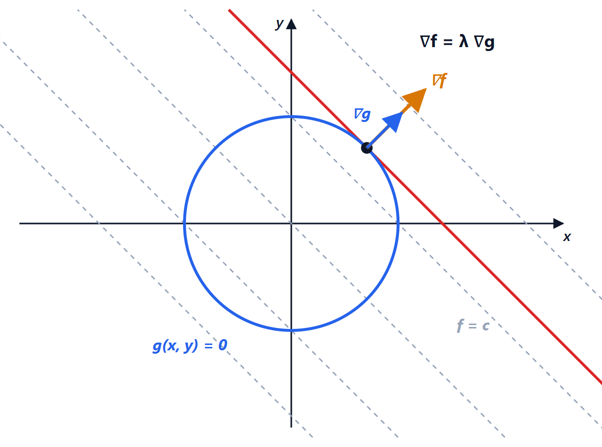
 on the circle
 . The dashed lines are the level curves of ; the red one is the last that still touches the circle, and it is tangent to it. At that point
 and
 are parallel.
Two tangent curves share the same normal line. The gradients are perpendicular to their level curves, so at the point of tangency and are parallel:

for some number  , the Lagrange multiplier.
Proof
Assume  . Then, by the implicit function theorem, near
 the constraint is a smooth curve that can be parametrised by
 ,
 . The function
 has an extremum at
 , so by the chain rule
 : the gradient of is perpendicular to the tangent of the constraint. So is
 , because
 for every
 and therefore
 . In the plane, two vectors perpendicular to the same direction are parallel.
The method
Define the Lagrangian

and look for its critical points, that is solve the system

Three equations in three unknowns. The solutions include every constrained extremum (along with any points where  , to be checked separately). If the constraint is a compact set, like a circle, the maximum and minimum exist by Weierstrass: just compare the values of at the candidates.
The example in the figure. ,  :
 ,
 , so
 , and from the constraint
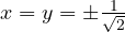 . Maximum
 at
 , minimum
 at the opposite point.
Example: the box of largest volume
A closed box shaped like a rectangular block must have surface area  m². What is the largest volume
 ? With the Lagrangian in three variables:

Multiplying the first by  and the second by
 :
 , so
 and . In the same way
 . The best box is a cube:
 , side 1 m, volume 1 m³.
The meaning of the multiplier
is not just an auxiliary unknown. If the constraint is  , the optimal value
 changes with
 , and

The multiplier says how much the optimum improves if the constraint is relaxed by one unit. In economics it is called the “shadow price” of the resource; in physics, in problems with mechanical constraints, the multipliers are the constraint forces.
Several constraints and inequalities
With several constraints  there is one multiplier for each:
 . For example, the extrema of a function on a curve in space, the intersection of two surfaces.
When the constraint is an inequality,  , as in the search for absolute extrema on a disc, interior points (zero gradient) and the boundary (Lagrange) are studied separately. The systematic generalisation is the Karush-Kuhn-Tucker conditions, the basis of the numerical optimisation used in circuit design and machine learning.
An electronics example: maximum power transfer
A voltage source  with internal resistance
 drives a load
 . The power in the load is
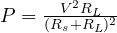 . Here the problem is unconstrained in one variable:
 gives
 , with maximum power
 . If instead the current may not exceed a maximum value, the constraint becomes active and the optimum moves to the edge of the allowed region: exactly the situation that calls for the methods of this lesson.