The definite integral: fundamental theorem, areas and applications in circuit theory
Riemann sums, properties, mean value theorem, fundamental theorem of calculus, areas between curves, charge, energy, mean and RMS values, numerical integration.
The definite integral starts from a geometric question, how large is the area under a graph, but it answers many physical ones: the charge carried by a current, the energy absorbed over a time interval, the mean and RMS value of a signal. The fundamental theorem of calculus connects it to antiderivatives and makes it computable.
Definition with Riemann sums
Split  into
 small intervals of width
 , choose a point
 in each and add up the areas of the rectangles:
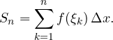
If, as the subdivision gets finer,  tends to the same limit whatever points are chosen,
 is integrable and the limit is
 . Continuous functions are integrable, and so are functions with finitely many jumps. Areas below the
 axis count with a minus sign.
Properties
- Linearity:
 .
- Additivity:
 .
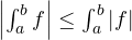
- Monotonicity: if
 then
 ; in particular
 .
- Symmetry: if is odd,
 ; if it is even,
 .
Mean value theorem for integrals
If is continuous on there is  such that
 . The quantity
 is the mean value of : in electronics it is the DC component of a signal.
The fundamental theorem of calculus
Let be continuous. The integral function  is differentiable and
 : the integral is an antiderivative. Consequently, if
 is any antiderivative,

Example:  . Without this theorem you would need to compute a limit of sums every time.
With a substitution the limits change too:  , with
 , becomes
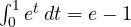 . By parts:
 .
Areas
The area between two graphs with  on is
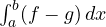 . For the area between
 and
 : the curves meet at 0 and 1, and on that interval
 , so the area is
 . If a function changes sign and you want the geometric area, integrate
 , that is split the interval at the points where vanishes.
Applications in circuit theory
- Charge:
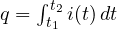 . The voltage across a capacitor is
 .
- Energy:
 . The energy stored in a capacitor charged to
 is
 .
- RMS value:
 . For
 it gives
 : the 230 V of the European mains are an RMS value, with a peak of about 325 V.
- Mean value of a full-wave rectified sine:
 .
A longer physical application, the charge and discharge of a capacitor studied with integration, is in the in-depth article linked to this syllabus topic.
Numerical integration (outline)
When the antiderivative is not elementary, go back to the definition: the trapezoidal rule replaces rectangles with trapezoids, Simpson’s rule with parabolic arcs. With Simpson and only 10 intervals,  , already correct to five decimal places.