Functions of several variables: domain, level curves, limits and continuity
Topology of R^n, graphs and level curves, limits with examples of non-existence along lines and parabolas, polar coordinates, continuity and Weierstrass' theorem.
The temperature in a room depends on three coordinates, the resistance of a thermistor on temperature and current, the gain of an amplifier on frequency and load. Almost every real quantity depends on several variables. In this lesson we extend the ideas of Analysis 1 to functions  : how they are represented, what neighbourhoods, open and closed sets are, and how limits and continuity are defined.
The space 
The points of are  -tuples
 . Distance is Euclidean,
 . The ball (or neighbourhood) with centre
 and radius
 is
 : an interval in
 , a disc in the plane, a solid sphere in space.
Relative to a set  , a point can be:
- interior: there is a ball around it entirely inside ;
- boundary: every ball around it contains points of and points outside ;
- accumulation point: every ball around it contains points of other than itself.
is open if all its points are interior (the disc without its edge), closed if it contains its whole boundary (the disc with its edge), bounded if it fits inside a ball. A closed and bounded set is called compact: it is the counterpart of the intervals  of Analysis 1, and Weierstrass’ theorem still holds on it.
Representing a function of two variables
The graph of  is the surface
 in space. Since surfaces are awkward to draw, level curves are used: the sets
 , projected onto the
 plane. It is exactly the method of topographic maps (contour lines), weather maps (isobars) and electric field maps (equipotential lines).
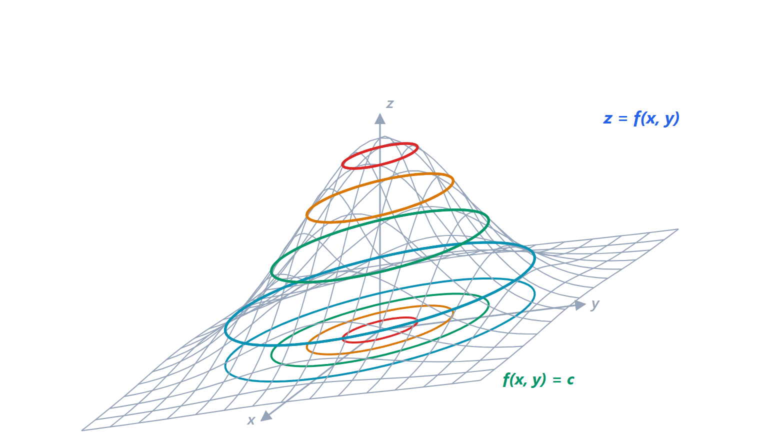 and some of its level curves: cutting the surface at constant heights gives curves which, projected onto the plane, form the function’s “contour map”.
Where the level curves (at equally spaced heights) are close together the function rises quickly; where they are far apart the surface is almost flat.
Examples.  has concentric circles as level curves and a paraboloid as graph.
 has hyperbolas as level curves and a “saddle” as graph.
 has parallel lines and a plane as graph.
Domain. As in Analysis 1 you need to find where the expression makes sense, but now the result is a region of the plane. For  you need
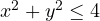 and
 : the disc of radius 2 intersected with the half-plane above the diagonal.
Limits
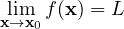
if for every  there is
 such that
 for all
 in the domain with
 . The definition is identical to Analysis 1, but with a huge difference: in the plane you can approach the point from infinitely many directions and along infinitely many paths, and the limit must be the same for all of them.
How to show a limit does not exist
It is enough to find two paths along which the limits differ. Example:

Along the  axis (
 ) it is always 0. Along the line
 it equals
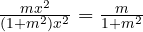 , which depends on
 : along the diagonal it is
 . The limit does not exist.
Careful: having the same limit along every line is not enough. For 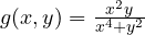 the limit along every line through the origin is 0, but along the parabola
 the function is constantly .
How to show a limit exists: polar coordinates
Set  ,
 , and look for a bound
 with
 , independent of
 . Example:

so the limit is 0. It is not enough that for each fixed the limit in  is zero: the bound must be uniform in , otherwise you fall back into the parabola case.
Continuity
 is continuous at if
 . Sums, products, quotients (where the denominator is non-zero) and compositions of continuous functions are continuous: polynomials in and
 ,
 ,
 are continuous everywhere.
The function  , extended by 0 at the origin, is not continuous at
 , even though it is continuous along every horizontal and vertical line: the first sign that things are more delicate in several variables.
Weierstrass’ theorem. A continuous function on a compact set has a maximum and a minimum. We will use it to look for absolute extrema in the lessons on maxima and minima.
Vector-valued functions
More generally one studies functions  . With
 they are curves (the position of a point as a function of time); with
 or
 they are vector fields, such as the electric field or the velocity of a fluid, which attach a vector to every point. Limits and continuity are studied component by component.