Fourier series: coefficients, convergence and signal spectra
Orthogonality and the coefficient formulas, the square wave and its harmonics, Dirichlet's theorem, the Gibbs phenomenon, Parseval's identity and the complex form.
The Taylor series approximates a function with powers, and it is excellent near a point. For periodic functions, such as the signals of a circuit in AC steady state, sines and cosines are far more natural. Fourier proposed this in 1807 to solve the heat equation; today it is the foundation of signal analysis, filters, audio compression and communications.
Trigonometric polynomials and Fourier series
We want to write a function  of period
 as

The term  is the mean value, the
 terms are the fundamental, those with
 the harmonics. For any period
 , replace
 with
 , where
 .
Proof: the coefficient formulas
The key is the orthogonality relations: for integers 

They are proved with product-to-sum formulas: for example  , and the integral over a period of
 is zero for every
 .
Multiply the series by  and integrate over
 , assuming we may integrate term by term. Every term vanishes except the one with , which gives
 . Hence

It is exactly the computation of coordinates in an orthogonal basis from the Geometry and Algebra lesson: the functions  and
 are an orthogonal basis for the inner product
 , and the Fourier coefficients are the projections of onto it.
Useful symmetries. If is even, all  are zero (a cosine series); if it is odd, all
 are zero (a sine series).
Example: the square wave
Let  for
 and
 for
 , extended periodically. It is odd, so
 , and


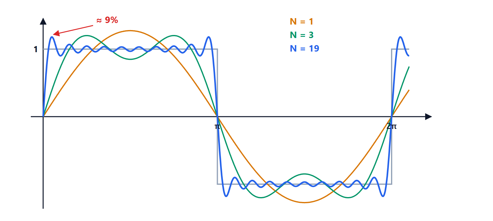
A square wave contains only odd harmonics, with amplitude falling as  . That is why a 100 MHz digital clock produces interference at 300, 500, 700 MHz, and why the edges of fast signals are sometimes deliberately slowed down.
Convergence
Theorem (Dirichlet). If is periodic and piecewise smooth (with finitely many jumps and corners in a period), the Fourier series converges at every point:
- to
 where is continuous;
- to the average
 at jumps.
For the square wave, at  the series gives 0, the average of
 and
 .
Near the jumps the convergence is not uniform: the partial sums overshoot the function by about 9% of the size of the jump, and this peak moves towards the jump but does not shrink as terms are added. This is the Gibbs phenomenon, visible in the figure. If instead is continuous and piecewise smooth, the convergence is uniform.
Parseval’s identity and energy

It is Pythagoras’ theorem in infinite dimensions: the squared norm is the sum of the squares of the coordinates. Physically, the power of a periodic signal is the sum of the powers of its harmonics. For the square wave the left side is 2, and a surprising result follows:  , that is
 .
It also follows that the fundamental alone carries 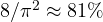 of the square wave’s power: this is the starting point for computing a signal’s total harmonic distortion (THD).
Complex form
With Euler’s formula the series becomes more compact:

This is the form used in electronics and telecommunications. Letting the period tend to infinity, the sum over discrete frequencies  becomes an integral over all frequencies: the Fourier transform, which describes the spectrum of non-periodic signals. The version for sampled signals, computed with the FFT algorithm, is inside every digital oscilloscope, modem and audio codec. The Z transform, linked to this subject, generalises it to discrete-time systems.