Solved exercises on Bode plots, Nyquist and stability margins
Nine exercises with solutions and plots: asymptotic Bode, resonant peak, margins, gain for a phase margin, delay margin, lead network, Nyquist of an unstable process, counting encirclements, non-minimum-phase zero.
Exercises on Bode plots, the Nyquist criterion and stability margins of the kind set in Control Systems courses, in three levels: basic, with drawing and reading plots by hand; intermediate, with margins, delays and gain design; exam, with open-loop unstable processes, counting encirclements, compensating networks and non-minimum-phase systems. The result is given straight away; the full solution, with the plot, opens with a click. The proofs and the MATLAB and Python code are in the in-depth study linked at the top.
Basic level
Exercise 1. Bode by hand
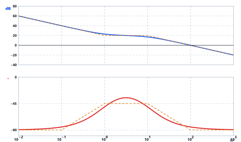
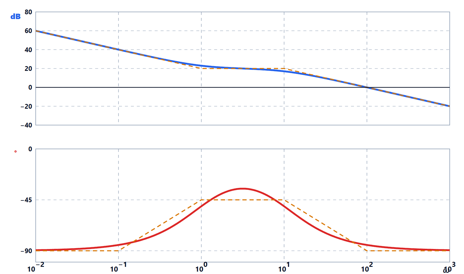
Draw the asymptotic Bode plots of  and estimate the crossover frequency and the phase margin.
Result: Bode form  ; crossover about 100 rad/s; phase margin about 95°.
Solution
Bode form (factors with constant term 1):  . Gain 10, one integrator, a zero at 1, a pole at 10.
Asymptotic magnitude. For  :
 , a line at −20 dB per decade that is 20 dB at
 . Between 1 and 10 the zero cancels the integrator: flat at 20 dB. After 10: again −20 dB per decade,
 , which is 0 dB at
 .
Phase. It starts from  (integrator), rises towards
 because of the zero, returns to after the pole. At :
 , so
 .
Exact values (with the code of the in-depth study):  rad/s,
 ; at the actual magnitude is 23 dB (the asymptote gives 20: the +3 dB error of the zero).
Exercise 2. The resonant peak
A second-order system has  rad/s and
 . Compute the resonant peak, the frequency at which it occurs and the phase at
 .
Result:  (8.1 dB) at
 rad/s; phase at .
Solution
From the in-depth study:  , i.e.
 dB.
 rad/s. At
 the denominator
 equals
 : phase , magnitude
 .
The peak in frequency and the step overshoot (52.7 % for ) are two faces of the same lack of damping: an instrument that measures the frequency response of a system allows  to be estimated from the peak.

Exercise 3. Reading the margins
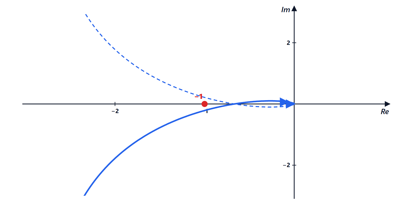
For 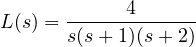 compute the gain margin by hand and check on the Nyquist plot that the closed loop is stable.
Result:  ,
 (3.5 dB);
 at 1.14 rad/s; stable, with small margins.
Solution
Phase  requires
 , i.e.
 (two complementary angles have reciprocal tangents): .
 , so : the critical gain is
 (the same that Routh gives on
 :
 ).
On the Nyquist plot,  has no poles in the right half-plane (
 ) and the curve crosses the negative half-axis at
 , without encircling
 :
 ,
 , stable.

Intermediate level
Exercise 4. The gain for a phase margin
For  find the gain that gives a phase margin of 45°. What is the gain margin then?
Result:  , with
 rad/s;
 (13 dB).
Solution
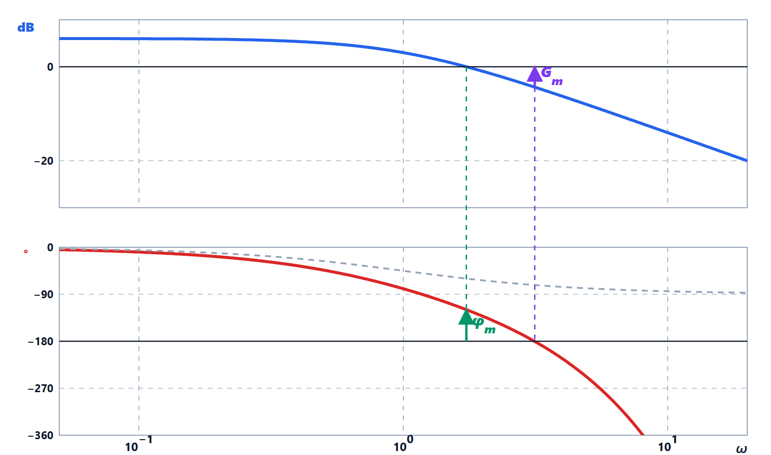
The gain does not change the phase. First find the frequency where the phase is  :
 . With the tangent addition formula:
 , i.e.
 ,
 .
Then choose  so that the magnitude there is 1:
 .
Gain margin: the critical gain is 6 (exercise 3), so  . The closed-loop overshoot turns out to be 24 %, consistent with the rule
 .
Exercise 5. How much delay can be tolerated
For 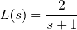 compute the phase margin and the maximum delay that can be inserted into the loop before instability.
Result:  ,
 ; maximum delay 1.21 s.
Solution
 for . Phase
 , margin
 .
A delay  adds
 to the phase without changing the magnitude: the crossover stays at
 , and instability arrives when
 rad, i.e.
 s.
Without delay the first-order system is stable for any gain; with a delay, it is not. This is why systems controlled over a network (vehicles, teleoperated robots) must take latency into account.
Exercise 6. A lead network
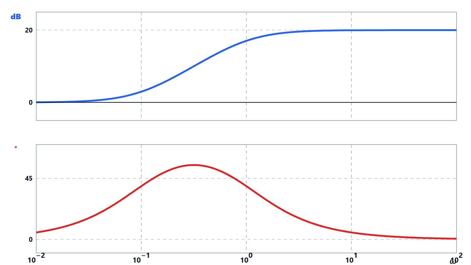
The network  is a lead network with
 . Find the maximum phase lead, the frequency at which it occurs and the gain at that point.
Result:  at
 rad/s; gain
 , i.e. 10 dB.
Solution
With  (here
 ), the phase is
 . Differentiating and setting to zero gives the maximum at the geometric mean of the two corner frequencies:
 .
There  ,
 , and
 (10 dB, half of the total 20 dB).
In design,  is placed at the new crossover frequency, to use all the lead where it is needed; the gain
 must be compensated.
Exam level
Exercise 7. Nyquist with an unstable process
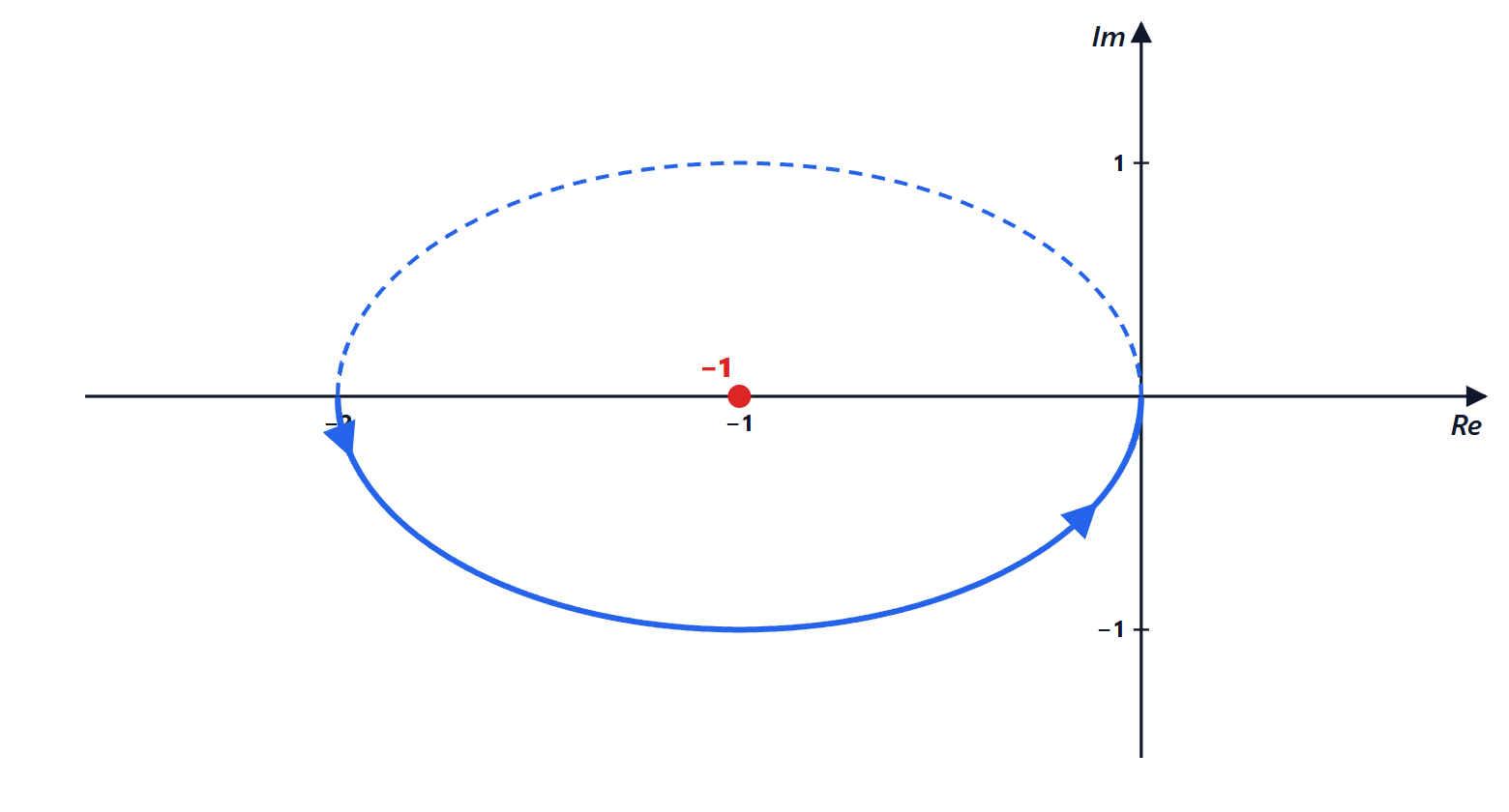
The process  has an unstable pole. Draw the Nyquist plot for
 and use the criterion to determine for which the closed loop is stable.
Result: stable for  ; for the plot encircles once anticlockwise.
Solution
 . For
 it is
 , for
 it tends to 0. Real and imaginary parts satisfy
 : a circle centred at
 with diameter from to 0.
The process has  . If the circle contains , traversed (for
 from
 to
 ) anticlockwise:
 , so
 , stable. If
 , stays outside: ,
 , unstable.
Direct check: the closed loop has pole  , negative for . With an unstable process, the plot must go round , in the right direction, for the loop to be stable.
Exercise 8. Counting encirclements
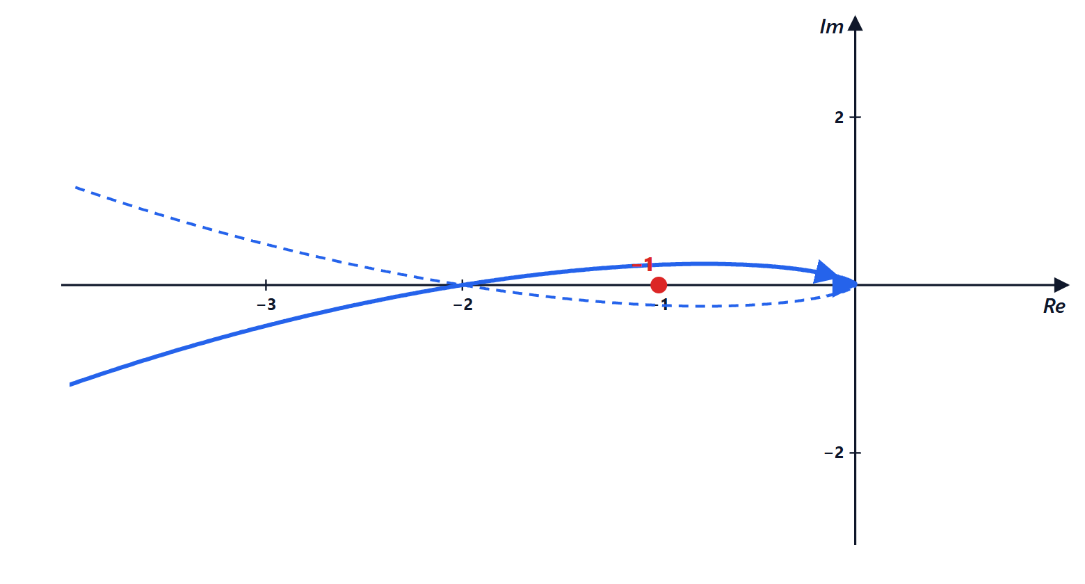
For  use the Nyquist criterion to count the unstable closed-loop poles.
Result: two clockwise turns round :  , closed loop unstable with a pair of poles in the right half-plane.
Solution
From the lesson, for  the plot crosses the negative half-axis at
 at the frequency
 . With
 the crossing is at
 , to the left of .
Following the complete curve (for positive and negative , closed at infinity clockwise because of the integrator), the point is encircled twice clockwise:  . The process is stable, , so .
Check with Routh on  :
 , two sign changes in the first column, two unstable poles.
Exercise 9. A non-minimum-phase zero
The system 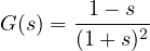 has a zero at
 . Compute the step response, its minimum value and the time at which it is reached, and compare the phase with that of
 .
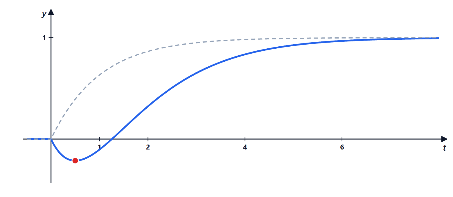
Result:  ; minimum
 at
 s; the phase falls to
 instead of stopping at .
Solution
 (residues: at 0 it is 1; for the double pole,
 ,
 ,
 ). So
 .
 : negative for
 . The response starts downwards, reaches
 and then rises towards 1.
In frequency:  , same magnitude; but
 instead of
 . The total phase goes from 0 to . The extra phase lag reduces the margin and limits the achievable bandwidth: with an unstable zero at
 , the crossover frequency cannot exceed about
 .