Random processes, power spectral density and thermal noise
Stationarity and ergodicity, power spectral density, passing through a filter with proof, white noise, thermal noise, kT/C noise with proof, shot and 1/f noise.
A random variable describes an uncertain number; a random process describes an entire uncertain signal, a random value at every instant. The noise of a circuit, speech, transmitted data are random processes. Their waveform cannot be predicted, but one can compute their power, how it is spread over frequency and how a filter changes it. In this lesson we cover these tools and apply them to thermal noise.
Random processes
A process  can be thought of as the set of all the waveforms an experiment could produce (the realisations). At a fixed instant,
 is a random variable. The main quantities are

the mean and the autocorrelation, which says how closely the values at two different instants are related.
Stationarity. A process is wide-sense stationary if its mean is constant and its autocorrelation depends only on the distance between the instants:  . Its statistical properties do not change over time.
 is the average power.
Ergodicity. A process is ergodic if time averages over a single long realisation coincide with ensemble averages. This is the assumption always made in practice: you measure the noise of one amplifier for a long time, not of a thousand amplifiers at the same instant.
Power spectral density
Definition (Wiener-Khinchin). For a stationary process, the power spectral density is the Fourier transform of the autocorrelation:

Inverting at  :
 . The total power is the area under
 , and the power in a band is the area over that band: is measured in W/Hz (or V²/Hz).
Passing through a filter
Theorem. If a stationary process  passes through a stable LTI system with frequency response
 , the output
 is stationary and

Proof. The output is  . Then

which depends only on  . The expression is the convolution of
 with
 and with
 . Transforming, convolution becomes a product and the transform of is
 (real response):
 . ∎
The filter’s phase does not matter: for power only the magnitude counts.
White noise
A process with constant spectral density,
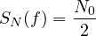
is called white noise, by analogy with white light, which contains all colours. Its autocorrelation is  : two values at different instants, however close, are uncorrelated. It is an idealisation (it would have infinite power), but an excellent model as long as the noise bandwidth is much wider than that of the system receiving it. If it is also Gaussian it is called additive white Gaussian noise (AWGN), the standard model of communication channels.
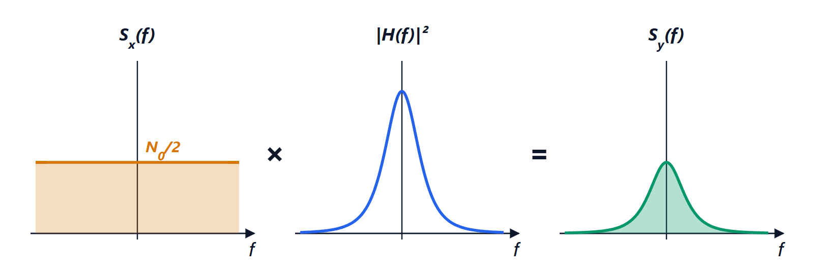
At the output of a filter the noise power is  . The noise equivalent bandwidth
 is defined as the bandwidth of the ideal filter with the same peak gain that passes the same power: for an RC low-pass,
 .
Thermal noise
The electrons of a resistor jiggle because of temperature, and a noise voltage appears across it. Johnson and Nyquist’s result (1928) is that, up to very high frequencies, it is white Gaussian noise with
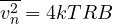
in a bandwidth  , where
 J/K is Boltzmann’s constant and
 the absolute temperature.
Example. A 1 kΩ resistor at 300 K, over the 20 kHz audio band:  µV. It seems small, but it is the floor below which no microphone or sensor connected to that resistance can be amplified without noise.
Theorem (kT/C noise). The noise voltage across the capacitor of an RC circuit has power

independent of R.
Proof. The resistor noise, with density  over positive frequencies only, passes through the RC divider:
 . Integrating:

using 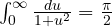 . ∎
A larger resistance makes more noise, but it also narrows the bandwidth in the same proportion. With  pF,
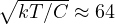 µV: it is the fundamental noise of switched-capacitor circuits and of image sensor pixels, and the reason the sampling capacitors of precision converters cannot be too small.
Other noises
- Shot noise: the current in a junction is made of discrete charges crossing it at random; it is white with
 .
- 1/f noise (flicker): a spectral density that grows at low frequencies, due to defects in materials; it dominates in MOSFETs below a few kilohertz.
- Markov processes: in many systems (packet queues, channels with burst errors) the future depends only on the present state; Markov chains are the basic model to describe them.





