Correlation: autocorrelation, Wiener-Khinchin, radar and GPS
Autocorrelation and its properties with proof, the Wiener-Khinchin theorem, cross-correlation and delay estimation, radar, Barker codes, GPS and the matched filter.
How similar are two signals? And how similar is a signal to itself shifted in time? Correlation answers these questions, and it is the tool with which a radar measures distance, a GPS receiver computes position, a modem synchronises and a system recognises a known signal buried in noise. In this lesson we cover autocorrelation, its properties, its link with the spectrum and cross-correlation.
Autocorrelation
For an energy signal (real, for simplicity) the autocorrelation is

Shift the signal by  , multiply it by the original and compute the area: if the two copies overlap well the product is mostly positive and the area is large, otherwise positive and negative contributions cancel.
Properties.
 : at zero the autocorrelation is the energy;
 : it is even;
 : the maximum is at zero.
Proof of the last one. By the Cauchy-Schwarz inequality for integrals,  . With
 and
 , both integrals under the roots equal
 , because shifting a signal does not change its energy:
 . ∎
No shifted copy resembles the signal more than the signal itself. The width of the central peak says how quickly the signal “forgets” itself: narrow for signals that change quickly (wide bandwidth), wide for slow signals.
The link with the spectrum
Theorem (Wiener-Khinchin, for energy signals). The Fourier transform of the autocorrelation is the energy spectral density:

Proof. With the change of variable  one sees that
 , that is the convolution of
 with
 . The transform of is
 for a real signal, and by the convolution theorem
 . ∎
Autocorrelation loses phase information: different signals with the same amplitude spectrum have the same autocorrelation.
Power signals. For periodic and random signals the time average is used,  . Then
 is the power and the transform is the power spectral density. The autocorrelation of a periodic signal is periodic with the same period: it is used to measure the pitch of a musical note (the first peak after zero) even when the signal is noisy.
Cross-correlation
Between two different signals:

If  contains a delayed copy of
 ,
 , the cross-correlation peaks exactly at
 : the first term gives
 , largest where copy and original line up, while the noise, which does not resemble , gives a small random contribution.
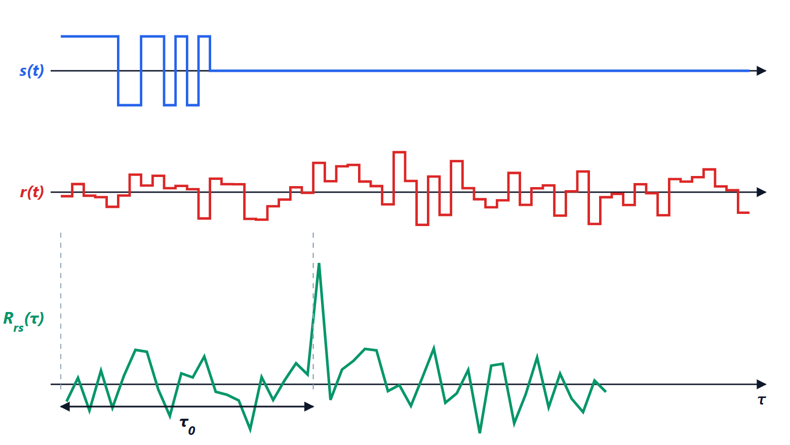
Radar. A pulse is transmitted and the received echo is correlated with the transmitted pulse: the peak gives the delay  , and the distance is
 (there and back). The resolution depends on the width of the peak, that is on the bandwidth: a 1 µs pulse separates targets at least about 150 m apart.
Pulse compression. A short pulse gives good resolution but little energy, hence short range. So a long but “coded” signal is transmitted, for example the 13-element Barker code in the figure, whose autocorrelation has a peak of 13 and side lobes of magnitude at most 1: the energy of a long pulse with the resolution of a short one.
GPS. Each satellite transmits a different pseudo-random code, 1023 elements long. The receiver correlates the received signal with local copies of the codes: the peaks say which satellites are visible and with what delay their signals arrive, and the position is computed from the delays. The GPS signal reaches the ground below the noise level, and correlation brings it out.
Correlation and convolution
The two operations are similar: correlation is a convolution with one of the two signals flipped,  . So correlating with is the same as passing the signal through a filter with impulse response
 , or
 to make it causal. This is the matched filter, which in the lesson on detection we will prove to be the best possible for recognising a known signal in white noise.