Waveforms and pulse compression: matched filter proved, chirp, Barker codes and ambiguity function

The radar equation asks for energy to see far; range resolution asks for bandwidth, that is short pulses. With a simple pulse of duration the two requirements conflict: a short pulse carries little energy, unless the peak power is huge. Pulse compression resolves the conflict: a long pulse is transmitted, but with an internal modulation that makes it “wide in bandwidth”, and in reception it is compressed by a matched filter. This lesson proves that the matched filter is the optimum receiver, analyses the linear chirp and the Barker codes, and introduces the ambiguity function, which describes at once the range and velocity resolution of any waveform.

The idea in simple words

Imagine having to recognise a friend’s whistle in a noisy room. If the whistle is a very short sharp blast, it gets lost in the noise. If instead it is a long tune you know well, you recognise it even when it is faint: your brain compares what it hears with the tune it expects, note by note, and adds up all the small similarities. This is exactly what the matched filter does: it compares the received signal with a copy of the transmitted one, instant by instant, and gives a peak when the two match.

The chirp is the most used “tune”: a whistle whose pitch rises steadily, like a bird’s song (hence the name). The radar transmits a long chirp, hence with plenty of energy; when the receiver compares it with the copy, all that energy is concentrated in a very narrow peak, as if the radar had transmitted a very short and very powerful pulse. Range (energy) and precision (narrow peak) are obtained together.

The matched filter

The receiver gets , with the expected echo and white noise of spectral density . We look for the linear filter that maximises the output signal-to-noise ratio at an instant .

Theorem (matched filter). The optimum filter is , the time-reversed and conjugated replica of the signal, and the maximum signal-to-noise ratio is , with the signal energy.

Proof. At the output, in the frequency domain, the signal is and the noise power is . By the Cauchy-Schwarz inequality , hence

Equality holds if , which in time is . ∎

The result is remarkable: the optimum signal-to-noise ratio depends only on the energy of the signal, not on its shape. The shape can therefore be chosen to obtain the desired resolution, without losing sensitivity. Filtering with is the same as computing the correlation between the received and the transmitted signal: the output peaks at the echo delay.

The linear chirp

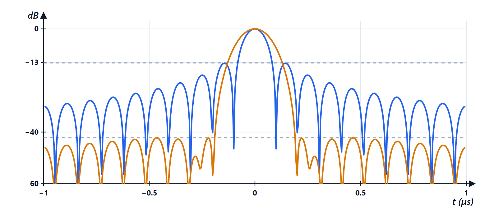
The chirp (linear frequency modulation, LFM) is a pulse of duration whose frequency rises linearly by : for . After the matched filter the compressed pulse has the shape of a sinc about wide (at −3 dB, ): the resolution is that of a pulse of duration , with the energy of a pulse of duration . The compression ratio is , the duration × bandwidth product.

Example. μs and MHz: . The compressed signal has a −3 dB width of 85 ns (against ns from theory: the small difference is due to sampling) and a resolution of 12.7 m, while the transmitted pulse is 3 km long. With the same peak power, a simple 85 ns pulse would carry 235 times less energy.

Sidelobes. The sinc has sidelobes at −13.2 dB: a strong echo can hide a weak target nearby. A window (Hamming, Taylor) is applied to the receive filter: with the Hamming window the sidelobes drop to −42 dB, at the cost of a wider peak (135 ns instead of 85, about 60 % more) and a small loss of gain. It is the same trade-off as windows in spectral analysis.

The chirp has two valuable practical properties: it is easy to generate (with voltage-controlled oscillators or direct digital synthesis) and it is Doppler tolerant: an echo from a moving target is still well compressed, only slightly shifted in range (the range-Doppler coupling). It is the waveform of the FMCW car radars (lesson on FMCW radars).

Phase codes

Alternatively the pulse is split into sub-pulses (“chips”) with phase 0 or π according to a code. Barker codes have the ideal autocorrelation for binary sequences: peak and sidelobes of magnitude at most 1. The longest known has length 13:

with autocorrelation and therefore a peak-to-sidelobe ratio of dB. For larger compression ratios, polyphase codes (Frank, P4) or long pseudo-random sequences are used, and in modern digital radars waveforms designed by computer.

The ambiguity function

The matched filter is matched to an echo with a given delay and a given Doppler. If the echo has a different Doppler , the output changes. Woodward’s ambiguity function describes the output as a function of both:

is the range response (the compression), the velocity response. A theorem by Woodward states that the volume 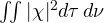is the same for all waveforms with the same energy: the ambiguity cannot be squeezed into a single point, only moved elsewhere. The chirp has a “tilted ridge” function (the range-Doppler coupling); a pulse train has a “bed of nails” function, with the range and velocity ambiguities of the lessons on the radar equation and on Doppler. Choosing the waveform is therefore choosing which ambiguities are acceptable for the application.

Summary

• The matched filter is the best possible receiver for a known signal in noise: it compares what is received with the copy of what was transmitted (correlation).
• The signal-to-noise ratio it achieves depends only on the signal energy, not on its shape.
• A long modulated pulse (chirp or phase code) carries plenty of energy and, after compression, gives the resolution of a short pulse: .
• The sidelobes of the compressed peak are lowered with a window, at the cost of a slightly wider peak.
• The ambiguity function shows how each waveform responds to range and velocity errors together; total ambiguity cannot be removed, only moved.

The code

import numpy as np

fs, T, B = 200e6, 20e-6, 10e6                       # sampling rate, chirp duration and bandwidth
t = np.arange(0, T, 1 / fs)
chirp = np.exp(1j * np.pi * B / T * (t - T / 2) ** 2)
received = np.r_[np.zeros(4000), chirp, np.zeros(4000)]          # isolated echo, no noise

def compress(window):
    y = np.abs(np.correlate(received, chirp * window, mode="same"))   # matched filter = correlation
    return y / y.max()

for name, w in (("rectangular", np.ones(len(chirp))), ("Hamming", np.hamming(len(chirp)))):
    p = compress(w)
    k = np.argmax(p)
    above = np.where(p >= 1 / np.sqrt(2))[0]                       # samples above -3 dB
    width = (above[-1] - above[0] + 1) / fs
    guard = int((1.5 if name == "rectangular" else 2.5) * fs / B)
    lobes = np.r_[p[:k - guard], p[k + guard:]]
    print(f"{name:12s}: -3 dB width {width * 1e9:.0f} ns, first sidelobe {20 * np.log10(lobes.max()):.1f} dB")
print(f"compression ratio BT = {B * T:.0f}, resolution c/(2B) = {3e8 / (2 * B):.0f} m")

barker = np.array([1, 1, 1, 1, 1, -1, -1, 1, 1, -1, 1, -1, 1])
print("Barker 13:", np.correlate(barker, barker, "full"), f"peak/sidelobe = {20 * np.log10(13):.1f} dB")

Running it prints 85 ns and −13.5 dB (rectangular), 135 ns and −42.2 dB (Hamming), and 15 m, and the autocorrelation of the Barker code with peak 13 and sidelobes 0 and 1.