The FMCW car radar: chirp and beat, velocity across chirps, virtual MIMO array and range-velocity map
How a 77 GHz radar measures range, velocity and angle: the beat frequency proved, resolution and range, velocity from the phase across chirps, the virtual MIMO array, the simulation of a frame with a double FFT.
Radar is one of the main sensors of modern cars: adaptive cruise control, automatic emergency braking, blind-spot monitoring and rear cross-traffic alert use it, and a car with driver assistance often has five or more. Unlike cameras it works in the dark, in fog and in rain, and it measures velocity directly. Almost all automotive radars are FMCW (frequency modulated continuous wave) at 77 GHz, built on a single chip with printed antennas. This lesson derives how an FMCW radar measures range, velocity and angle, proves the resolution and range formulas, explains the virtual MIMO array, and simulates a complete frame with double-FFT processing.
The idea in simple words
An FMCW radar does not transmit pulses: it transmits all the time, but with a frequency that rises continuously, like a siren rising in pitch. When the echo comes back it is the “siren” of a few instants earlier, so it has a slightly lower pitch than what the radar is emitting at that moment. The farther the target, the “older” the echo and the larger the pitch difference. The radar mixes the two signals and listens to the difference, the beat: a low tone, of a few megahertz, whose frequency gives the range directly.
For velocity the same trick as in the lesson on Doppler is used: the chirp is repeated many times and one looks at how the phase of the beat turns from one chirp to the next. For angle, the phases received by adjacent antennas are compared. Three FFTs (one for range, one for velocity, one for angle) turn the raw samples into a map of everything in front of the car.
The chirp and the beat
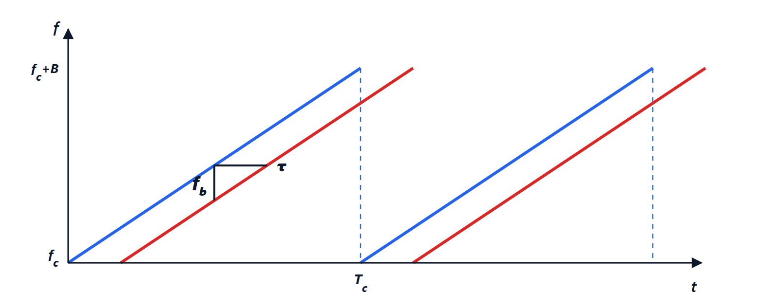
The radar continuously transmits a series of chirps: the frequency rises linearly from  to
 in a time
 , with slope
 . The echo of a target at range
 returns with a delay
 , so at every instant it has a slightly lower frequency than the one being transmitted. The receiver multiplies the echo by the transmitted signal (a mixer) and obtains the difference of the two frequencies, the beat signal.
Theorem. The beat frequency is 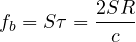 : proportional to range.
Proof. The phase of the transmitted signal is  . The echo is the same signal delayed by
 :
 . The mixer gives the phase difference:
 . The time-varying part is
 : a sinusoid of frequency
 . The constant terms give an initial phase
 (which will be used for velocity) and a negligible term. ∎
Range is therefore measured with an FFT of the beat: each target becomes a peak at a different frequency. With an ADC sampling at  (in quadrature), the maximum measurable frequency gives the maximum range
 , and the resolution of the FFT over one chirp (
 in frequency) gives the range resolution
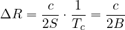
independent of the chirp duration: only the bandwidth counts. With  MHz, 25 cm; high-resolution parking radars use up to 4 GHz (3.75 cm) in the 77-81 GHz band. The beat is at a few megahertz: a target at 30 m with
 MHz/μs gives 2.4 MHz. This is a great practical advantage: a 77 GHz signal is processed with a cheap ADC at a few megahertz.
Velocity: from one chirp to the next
The Doppler shift of a car (a few kilohertz) is small compared with the beat frequency, and within a single chirp it is confused with range. It is measured instead across chirps, as in the pulse-Doppler of the lesson on Doppler.
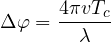
Theorem. Between two consecutive chirps, separated by , the beat phase of a target with radial velocity  changes by
 ; hence with
 chirps velocity is measured with an FFT, with resolution
 and unambiguous span
 .
Proof. The constant phase of the beat is  . In a later chirp the target has moved by
 , so the phase has changed by
 . The sequence of phases is a sinusoid along the chirps with frequency
 (the Doppler), sampled at : the FFT over samples has resolution
 in frequency, that is
 in velocity, and is unambiguous as long as
 , that is
 . ∎
At 77 GHz ( mm) with
 μs and 128 chirps: 0.30 m/s resolution, ±19.5 m/s without ambiguity (higher velocities are resolved with chirps of different durations, or with tracking). Arranging the samples in a matrix (rows: chirps; columns: samples of the chirp) and computing one FFT along the columns and one along the rows gives the range-velocity map of the whole scene in a frame of a few milliseconds.
Angle and the virtual MIMO array
With several receive antennas, the echo reaches each with a different phase,  between antennas a distance
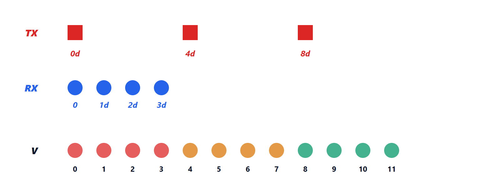
 apart (the phased-array geometry, lesson on phased arrays): a third FFT along the antennas gives the angle. Angular resolution grows with the number of antennas, but a chip has few channels. The trick is MIMO: with
 transmit antennas transmitting in turn (or with different codes), and
 receive antennas, each transmitter-receiver pair behaves as a “virtual” antenna at the position given by the sum of the two.
Property. If the transmit antennas are spaced  apart and the receive antennas apart, the virtual positions
 form a uniform array of
 elements with spacing .
Indeed the phase of the echo depends on the sum of the outbound path (from the transmit antenna) and the return path (to the receive antenna), that is on . With 3 transmit and 4 receive antennas, 12 virtual channels are obtained, with an angular resolution of about  radians, 9.5°; the latest “4D” radars, with tens of real channels, reach hundreds of virtual channels and also measure elevation (separating a bridge from a car stopped under it).
Simulating a frame
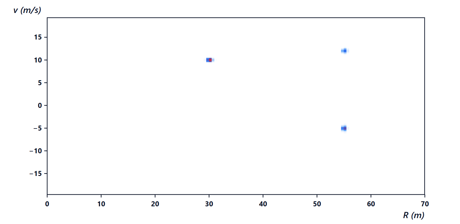
Radar at 77 GHz, MHz, μs, 512 samples per chirp, 128 chirps. Three targets: a car at 30 m moving away at 10 m/s, and at 55 m two objects at the same range, one approaching at 5 m/s and one moving away at 12 m/s (for example a car and a motorcycle side by side). The theoretical performance: 25 cm resolution, 128 m range, 0.30 m/s velocity resolution, ±19.5 m/s span.
The double FFT finds the three targets at (29.98 m; 10.04 m/s), (54.96 m; −5.17 m/s) and (54.96 m; 12.17 m/s): the true ranges and velocities, rounded to the grid cell. The two objects at 55 m, inseparable in range, are well separated in velocity: this is one of the reasons why radar recognises vehicles even in traffic.
Target configuration and real problems. Large objects (trucks, guardrails) give many points, small objects few; guardrails and stationary roadside objects are the main source of clutter; multipath (reflections off the road surface and vehicles) creates ghost targets; and with millions of equipped cars, interference between radars becomes a problem (another radar’s chirp crossing one’s own creates a disturbance pulse that raises the noise). The filtering of these effects is in the lesson on clutter, the construction of objects from points in the lesson that follows.
Summary
- The FMCW radar transmits frequency chirps; the beat between echo and transmitted signal has frequency
 , proportional to range.
- Range resolution is
 , only bandwidth counts; the maximum range depends on how the beat is sampled.
- Velocity is measured from the phase rotation across chirps: resolution
 , span
 .
- The virtual MIMO array multiplies the channels: elements with
 antennas.
- Double (or triple) FFT: the range-velocity(-angle) map of a frame in a few milliseconds.
The code
import numpy as np

c = 299792458.0
fc, B, Tc, Nc, Ns = 77e9, 600e6, 50e-6, 128, 512    # carrier, bandwidth, chirp duration, chirps, samples per chirp
S, lam = B / Tc, c / fc                              # chirp slope, wavelength
fs = Ns / Tc                                         # sampling rate (in quadrature)
t = np.arange(Ns) / fs
targets = [(30.0, 10.0, 1.0), (55.0, -5.0, 0.5), (55.0, 12.0, 0.3)]   # range, velocity, amplitude
rng = np.random.default_rng(0)

data = np.zeros((Nc, Ns), complex)                   # one row per chirp
for m in range(Nc):
    for R, v, a in targets:
        Rm = R + v * m * Tc                          # range changes from one chirp to the next
        data[m] += a * np.exp(1j * (2 * np.pi * 2 * S * Rm / c * t + 4 * np.pi * Rm / lam))
data += (rng.normal(size=data.shape) + 1j * rng.normal(size=data.shape)) * 0.05

rd_map = np.fft.fft(data * np.hanning(Ns), axis=1)                   # range FFT (along the chirp)
rd_map = np.fft.fftshift(np.fft.fft(rd_map * np.hanning(Nc)[:, None], axis=0), axes=0)   # velocity FFT
P = 20 * np.log10(np.abs(rd_map) + 1e-12); P -= P.max()

dR, dv = c / (2 * B), lam / (2 * Nc * Tc)
print(f"resolution {dR * 100:.0f} cm, range {Ns * dR:.0f} m, velocity resolution {dv:.2f} m/s, span +-{lam / (4 * Tc):.1f} m/s")
for _ in range(3):                                   # the three highest peaks
    i, j = np.unravel_index(np.argmax(P), P.shape)
    print(f"target: {j * dR:6.2f} m, {(i - Nc / 2) * dv:6.2f} m/s, {P[i, j]:5.1f} dB")
    P[max(0, i - 4):i + 5, max(0, j - 4):j + 5] = -200                # remove the peak found
print(f"beat at 30 m: {2 * S * 30 / c / 1e6:.2f} MHz; MIMO 3x4: {3 * 4} virtual channels, about {np.degrees(2 / 12):.1f} degrees")
Running it prints 25 cm, 128 m, 0.30 m/s and ±19.5 m/s, the three targets with 0, −7.2 and −11.6 dB, 2.40 MHz and 12 channels with 9.5°.





