Filtering clutter: clutter radar cross section, chaff, MTI and MTD, STAP, robust CFAR, sea, interference and jammers

In a real radar the echo of a target is almost always the smallest part of what is received. The ground, buildings, the sea, rain, flocks of birds, the guardrails of a motorway return much stronger echoes, the clutter; multipath creates ghost targets; other radars and jammers add interference. Much of the design of a radar consists in filtering all this without losing the targets. This lesson collects the techniques: the classification of clutter and how strong it is, Doppler filters (MTI, MTD, adaptive filters, STAP), amplitude filters (clutter maps and robust CFARs, with the problem of sea clutter), and the defence against interference and ghosts. Four simulations show the problems and the solutions with numbers.

Types of clutter

• Surface clutter (ground, buildings, sea): extended, tied to the illuminated cell, whose area grows with range; it is described by the coefficient (radar cross section per square metre), which depends on the grazing angle, the frequency and the polarisation. The ground is almost still; the sea moves with the waves.
• Volume clutter (rain, snow, chaff, that is clouds of metal strips dropped to confuse radars): it fills the whole cell and moves with the wind.
• Unwanted point echoes: birds, insects, wind turbines (which have their own Doppler and are a growing problem for air traffic radars), cars for a radar looking for aircraft.
• Multipath ghosts: the echo bounces off a surface (the sea, the road, the side of a truck) and arrives from a wrong direction or with a wrong range.

Two quantities summarise performance: the improvement factor (how much the signal-to-clutter ratio increases after the filter) and the subclutter visibility (how much weaker than the clutter a target can be and still be detected).

The idea in simple words

Looking for an aircraft with a radar is like looking for a firefly in front of a wall lit by a floodlight: the wall (ground, sea, rain) sends back much more light than the firefly. There are three ways to see it anyway: look only at what moves (Doppler filters: the wall is still, the firefly is not), know what the wall looks like and subtract it (clutter maps), or set the “something is there” threshold according to how bright the background around it is (CFAR). This lesson shows how radars combine the three.

How strong clutter is

Surface clutter. The illuminated cell at range , with a beam wide in azimuth and a pulse of duration , at low grazing angles is a rectangle of area . The clutter has a radar cross section . Example: surveillance radar with a 1.5° beam, a 1 μs pulse, ground with dB, at 20 km: m², m² (29 dBsm). An aircraft of 1-10 m² is therefore 19 to 29 dB below the clutter of its cell: without filters it cannot be seen. Since grows as and the clutter echo falls as , surface clutter falls as , more slowly than a target echo: the signal-to-clutter ratio worsens with range as , and does not improve by increasing power (which raises target and clutter alike). ranges from −40 dB (calm sea, desert, at low angles) to 0 dB and more (cities, mountains); a simple model is 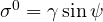, with the grazing angle.

Volume clutter. Rain and chaff fill the volume of the cell, , with a reflectivity (radar cross section per cubic metre). For rain , with for water and the reflectivity of the lesson on weather radars. In X band, with moderate rain of 30 dBZ, m²/m³: at 20 km, with a 1.5° × 1.5° beam and 1 μs, m³ and m², as much as an aircraft. Since goes as , in S band the same rain returns 21 dB less: another reason for using low frequencies for surveillance.

Chaff. Chaff is made of millions of wires or metallised strips cut to half a wavelength (1.5 cm in X band), resonant dipoles that return a lot of energy for their weight. A half-wave dipole with random orientation has on average : in X band m², so about 740 000 dipoles, a few grams of fibres, are needed to simulate a 100 m² target. The cloud opens in a few seconds, falls slowly and moves with the wind: the defence is the Doppler filter (chaff slows down at once and is distinguished from a fast aircraft), together with tracking, which does not let itself be “captured” by an echo that appears from nowhere and stays still. To cover several bands, wires of different lengths are cut.

The clutter spectrum. Clutter is not perfectly still: trees moved by the wind, sea waves, rain carried by the wind, and also the rotation of the antenna widen its Doppler spectrum. The spectrum is described by a velocity spread : from a few centimetres per second (rocks, buildings) to 0.5 m/s (woods in strong wind) to 1-2 m/s (sea, rain, chaff, plus the mean shift due to the wind). The wider the spectrum, the wider the notch of the MTI filter must be and the more slow targets are lost.

Doppler filters

Surface clutter is almost still, almost all interesting targets move: separating them in velocity is the main defence.

• MTI (lesson on Doppler): the canceller, or the three-pulse , removes what has zero Doppler. The improvement factor is limited by the width of the clutter spectrum (trees moved by the wind, antenna rotation, oscillator instability): clutter with a wide spectrum is not cancelled completely.
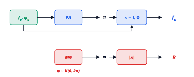
• MTD (moving target detector, the processor of airport approach radars): after the MTI, a bank of Doppler filters (an FFT over 8-16 pulses) splits the echoes by velocity, and each filter has its own CFAR threshold. For the zero-velocity filter, where clutter is strongest, a clutter map is used.
• Clutter map: the mean echo level of each cell over the previous antenna turns is stored (with an exponential moving average), and the threshold of each cell is a multiple of its level. An aircraft flying over an area of strong clutter is then seen if its echo exceeds the usual level of that cell, and targets flying tangentially (zero Doppler) do not disappear completely.
• Adaptive filters: rain, sea and chaff clutter moves with the wind, so its Doppler is not zero. An adaptive MTI estimates the mean Doppler of the clutter and moves the notch of the filter onto it.

STAP: clutter seen from an aircraft

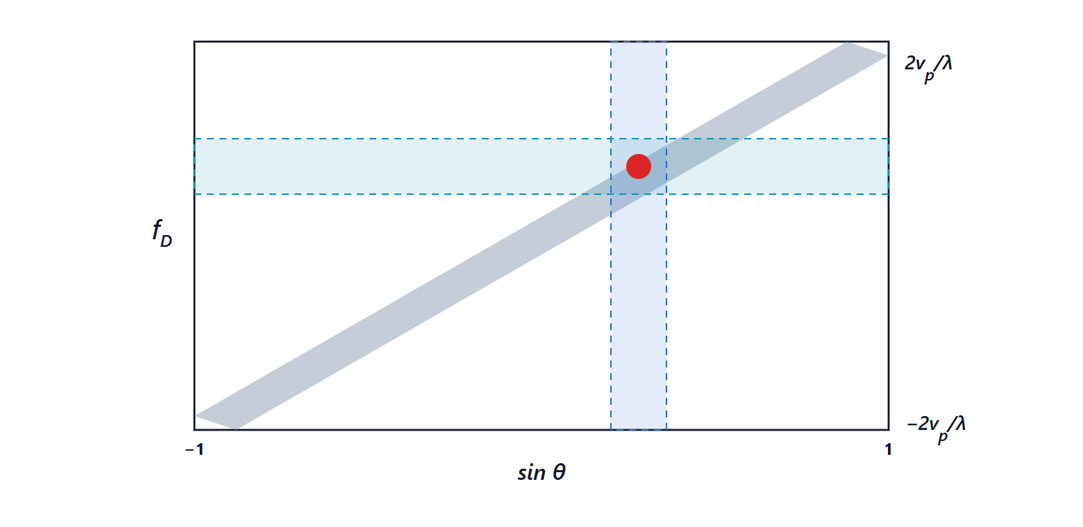
A radar on an aircraft or a satellite looking down sees the ground move: each patch of ground has a Doppler that depends on the direction it is seen from, (with the platform velocity). In the angle-Doppler plane the clutter occupies a diagonal ridge, and a filter in Doppler only or in angle only is not enough. STAP (space-time adaptive processing) filters jointly over the array elements (space) and the pulses (time), with the optimum weights

where is the covariance matrix of clutter, jamming and noise and is the “steering” vector of the target sought (angle and Doppler). These are the weights that maximise the signal-to-(interference + noise) ratio, SINR: the same Cauchy-Schwarz inequality as the matched filter, applied after “whitening” the interference with . In practice is unknown and is estimated from the data of neighbouring cells (SMI, sample matrix inversion): to lose less than 3 dB with respect to the optimum, about twice as many samples as degrees of freedom are needed (Reed, Mallett and Brennan rule). The same principle, in space only, serves to cancel a jammer: the adaptive array places a null of its pattern in the direction of the jammer.

CFAR in clutter: robustness

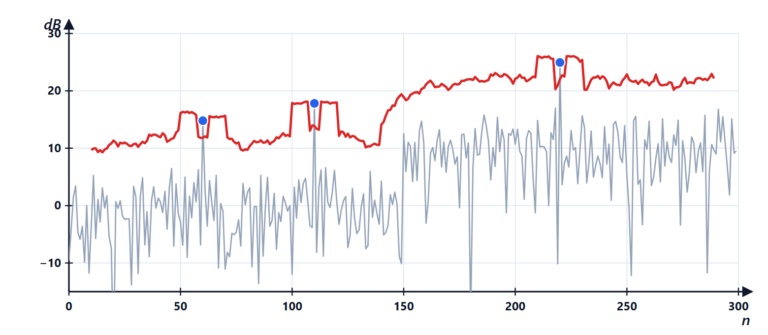
The CA-CFAR of the lesson on detection has two weak points:

• masking: if another target lies in the reference cells, the mean grows, the threshold rises and the target under test may disappear. It happens with close objects, such as two cars near each other or a formation of aircraft;
• clutter edges: at the transition between a quiet area and one of strong clutter (the shoreline, the edge of a rain cloud) the mean mixes the two levels: too many false alarms on one side, targets lost on the other.

The variants:

• OS-CFAR (order statistic): instead of the mean, the -th ordered value of the reference cells is used (for example the 12th out of 16). A few anomalous cells (another target) fall at the bottom of the ranking and do not count. For exponential noise , from which the threshold is obtained;
• GO-CFAR and SO-CFAR: the level is estimated separately to the left and right of the cell and the greater (against false alarms at edges) or the smaller (against masking) is taken.

Simulation 1. Two 18 dB targets 4 cells apart in noise, CFAR with 16 reference cells and 2 guard cells per side, , 300 trials. The CA-CFAR detects both targets only in 65 % of cases (the second raises the threshold of the first and vice versa); the OS-CFAR in 100 %. In noise only the two have the same false alarm rate: and .

Sea clutter and the tails of the distribution

The CFAR of the lesson on detection assumes a Gaussian background (Rayleigh amplitude, exponential power). Sea clutter, seen at grazing angles and with high resolution, is not: waves create short and intense spikes. It is described by the K distribution: a Gaussian “speckle” whose mean power fluctuates slowly from cell to cell according to a gamma distribution with shape parameter . The smaller , the “spikier” the sea; for the Gaussian case returns.

Simulation 2. A threshold computed for with the Gaussian model, applied to K clutter: with false alarms are (almost Gaussian), with 35 times more (), with 140 times more (). A naval radar that ignores the statistics of the sea fills up with false targets. The defences: thresholds computed on the K distribution estimated from the data, integration over several antenna turns (sea spikes are short-lived, a boat stays), and horizontal polarisation, which usually sees less sea clutter.

Interference and ghosts

• Interference between radars: in FMCW car radars, a chirp of another vehicle crossing one’s own produces, after the mixer, a short wideband pulse that raises the noise floor at all ranges and can hide weak targets. The countermeasures: detect the anomalous samples in time and zero them (or rebuild them by interpolation) before the FFT, randomise the chirp parameters, coordinate the radars.

Simulation 3. A weak target stands 35.9 dB above the noise floor. An interference of 30 samples out of 512 brings it down to 2.0 dB: invisible. Zeroing the samples with anomalous amplitude, the target comes back to 34.6 dB: only 1.3 dB is lost.

• Jammers (in military applications): a transmitter that floods the receiver with noise. The main defence is adaptive nulling with the array.

Simulation 4. An 8-element array at half a wavelength, target at broadside, jammer at 20° and 30 dB above the noise. With the fixed beam the jammer enters through a sidelobe at −13 dB and the SINR is −17 dB: the target is lost. With adaptive weights estimated from 64 samples (), the gain towards the jammer drops to −65 dB and the SINR rises to 8.2 dB, close to the theoretical maximum of 9.0 dB (, the gain of 8 elements in noise only).

• Multipath ghosts: a true target and its reflected image usually have the same radial velocity but positions geometrically incompatible with the terrain (for example below the road surface, or behind a guardrail). They are recognised with the known geometry, with tracking (the ghost “jumps” when the geometry of the reflection changes) and, in car radars, by comparison with the other sensors.

Summary

• Surface clutter has a radar cross section and often exceeds an aircraft echo by 20-30 dB; volume clutter (rain, chaff) grows with the cell volume and, for rain, as .
• Doppler filters (MTI, MTD, adaptive) remove what does not move; from an aircraft STAP is needed, working jointly in angle and Doppler.
• Clutter maps and robust CFARs (OS, GO) handle clutter edges and close targets; sea clutter has long tails (K distribution) and requires higher thresholds.
• Interference and jammers are fought by removing anomalous samples and by nulling the direction of the jammer with the array.

The code of the four simulations

import numpy as np

rng = np.random.default_rng(0)
dB = lambda x: 10 ** (x / 10)

# 1) CFAR: two close targets, the CA-CFAR "masks" the second, the OS-CFAR does not
def cfar(p, N=16, guard=2, pfa=1e-4, kind="CA", k=12):
    alpha = N * (pfa ** (-1 / N) - 1)                                   # CA-CFAR (lesson on detection)
    if kind == "OS":                                                    # threshold for the k-th order statistic
        a_lo, a_hi = 1.0, 100.0                                         # Pfa(alpha) = prod_{i=0}^{k-1} (N-i)/(N-i+alpha)
        for _ in range(100):
            a = (a_lo + a_hi) / 2
            pf = np.prod([(N - i) / (N - i + a) for i in range(k)])
            a_lo, a_hi = (a, a_hi) if pf > pfa else (a_lo, a)
        alpha = a
    det = []
    h = N // 2
    for i in range(h + guard, len(p) - h - guard):
        ref = np.r_[p[i - guard - h:i - guard], p[i + guard + 1:i + guard + 1 + h]]
        level = ref.mean() if kind == "CA" else np.sort(ref)[k - 1]
        threshold = alpha * level if kind == "OS" else alpha / N * ref.sum()
        det.append(p[i] > threshold)
    return np.r_[np.zeros(h + guard, bool), det, np.zeros(h + guard, bool)]

cells = 200
found = {"CA": 0, "OS": 0}
trials = 300
for _ in range(trials):
    p = rng.exponential(1.0, cells)
    p[100] += dB(18); p[104] += dB(18)                                  # two 18 dB targets 4 cells apart
    for t in ("CA", "OS"):
        d = cfar(p, kind=t)
        found[t] += d[100] and d[104]
print(f"two close targets both detected: CA-CFAR {found['CA'] / trials:.0%}, OS-CFAR {found['OS'] / trials:.0%}")
fa = {"CA": 0, "OS": 0}
for _ in range(50):
    p = rng.exponential(1.0, 4000)
    for t in ("CA", "OS"):
        fa[t] += cfar(p, kind=t).sum()
print(f"false alarms per cell in noise only: CA {fa['CA'] / (50 * 3960):.1e}, OS {fa['OS'] / (50 * 3960):.1e}")

# 2) sea clutter with K distribution: the "Gaussian" threshold gives too many false alarms
M = 2_000_000
for nu in (0.5, 2.0, 100.0):
    texture = rng.gamma(nu, 1 / nu, M)                                  # fluctuating local power (mean 1)
    power = texture * rng.exponential(1.0, M)                           # modulated exponential speckle: K clutter
    threshold = -np.log(1e-4)                                           # right threshold for Gaussian clutter
    print(f"K clutter with nu = {nu:5}: Pfa with the Gaussian threshold {np.mean(power > threshold):.1e} (wanted 1e-4)")

# 3) interference between FMCW radars: zeroing the corrupted samples lowers the noise
Ns = 512
t = np.arange(Ns)
signal = 0.2 * np.exp(1j * 2 * np.pi * 60 / Ns * t)                     # a weak target in bin 60
noise = (rng.normal(size=Ns) + 1j * rng.normal(size=Ns)) * 0.05
interf = np.zeros(Ns, complex)
interf[200:230] = 5 * np.exp(1j * np.pi * 0.02 * (t[200:230] - 215) ** 2)   # another radar's chirp crossing ours
def peak_over_floor(x):
    X = np.abs(np.fft.fft(x * np.hanning(Ns)))
    return 20 * np.log10(X[60] / np.median(X))
x = signal + noise + interf
xz = x.copy(); xz[np.abs(x) > 1.0] = 0                                  # detect and zero the anomalous samples
print(f"target above the floor: without interference {peak_over_floor(signal + noise):.1f} dB, with interference {peak_over_floor(x):.1f} dB, "
      f"after zeroing {peak_over_floor(xz):.1f} dB")

# 4) adaptive nulling: 8-element array, jammer at 20 degrees, target at broadside
Ne, d = 8, 0.5                                                          # spacing in wavelengths
steering = lambda th: np.exp(1j * 2 * np.pi * d * np.arange(Ne) * np.sin(np.radians(th)))
J = 1000.0                                                              # jammer 30 dB above the noise
samples = np.sqrt(J) * steering(20)[:, None] * (rng.normal(size=(1, 64)) + 1j * rng.normal(size=(1, 64))) / np.sqrt(2) \
          + (rng.normal(size=(Ne, 64)) + 1j * rng.normal(size=(Ne, 64))) / np.sqrt(2)
Rcov = samples @ samples.conj().T / 64                                  # estimated covariance (SMI)
w_ad = np.linalg.solve(Rcov, steering(0)); w_ad /= np.abs(w_ad.conj() @ steering(0))
w_fx = steering(0) / Ne                                                 # fixed beam towards the target
for name, w in (("fixed", w_fx), ("adaptive", w_ad)):
    g_t = np.abs(w.conj() @ steering(0)) ** 2
    g_j = np.abs(w.conj() @ steering(20)) ** 2
    noise_out = np.real(w.conj() @ w)
    print(f"{name:8s} beam: gain towards the jammer {10 * np.log10(g_j / g_t):6.1f} dB, "
          f"SINR {10 * np.log10(g_t / (J * g_j + noise_out)):6.1f} dB")

Running it prints all the numbers of the four simulations: 65 % and 100 % for the two CFARs, false alarms and , , and for K clutter, 35.9, 2.0 and 34.6 dB for the interference, and for the array −13 dB and −17 dB with the fixed beam, −65.5 dB and 8.2 dB with the adaptive one. The points left after filtering are used, in the dedicated lesson, to build objects.