Signals and systems: energy, power, LTI systems and convolution
Classifying signals, energy and power, elementary signals, system properties, convolution with proof and graphical computation, causality and BIBO stability.
A signal is a quantity that varies in time and carries information: the voltage from a microphone, the current in an antenna, the sequence of numbers read from a converter. A system is anything that turns one signal into another: a filter, an amplifier, a transmission channel, a program. Signal theory studies how to describe both and how to predict a system’s output. In this lesson we cover the basic definitions and the most important result: for linear time-invariant systems the output is a convolution.
Classifying signals
- Continuous-time
 or discrete-time
 , defined only at integer instants (for example the samples of a converter).
- Deterministic, described by a formula, or random, of which only the statistical properties are known (noise, but also speech or transmitted data, which are not known in advance).
- Periodic, with
 , or aperiodic.
Energy and power. The energy of a signal is
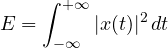
(the name comes from the case of a voltage across a 1 Ω resistor). A rectangular pulse of amplitude  and duration
 has energy
 . Signals that last forever, like a sinusoid, have infinite energy: for them the average power is used,
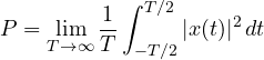
For  ,
 . A signal is an “energy signal” if
 is finite, a “power signal” if
 is finite.
Elementary signals
- the step
 , equal to 0 for
 and 1 for
 : a switch closing;
- the rectangular pulse
 , of duration ;
- the exponential
 , the response of first-order circuits;
- the sinc,
 , which appears in every band-limited problem;
- the Dirac delta
 , a pulse of zero duration and unit area, with the sifting property
 (Mathematical Methods lesson on the delta).
System properties
A system turns an input into an output  . The properties that matter:
- linearity: the response to
 is
 ;
- time invariance: if the input gives , the delayed input
 gives
 : the system does not change over time;
- causality: the output at an instant depends only on the input up to that instant;
- stability (BIBO, bounded input bounded output): every bounded input gives a bounded output.
Linear time-invariant (LTI) systems are the most important case: circuits with resistors, capacitors, inductors and linear amplifiers, digital filters, many transmission channels.
Convolution
The impulse response  is the system’s output when the input is .
Theorem. The output of an LTI system with impulse response  is the convolution of the input with :

Proof. By the sifting property, the input can be written as a “sum” of shifted, weighted impulses:
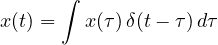
By time invariance, the response to  is
 . By linearity, the response to a combination (even a continuous one) of impulses is the same combination of the responses:
 . ∎
The result is powerful: an LTI system is completely described by a single function, its impulse response.
Graphical computation. To find  at an instant
 : flip (
 ), shift it by (), multiply it by
 and compute the area of the product. Sliding gives the whole output.
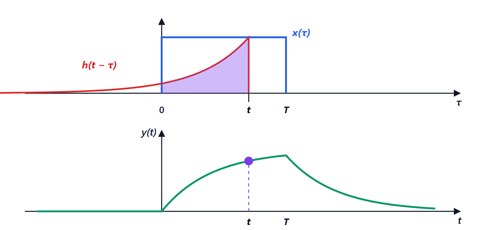
Example. An RC circuit with the output across the capacitor has  . With a rectangular pulse of duration at the input, the convolution gives an exponential charge for
 and an exponential discharge afterwards: exactly the curve in the figure, and it matches what one gets by solving the differential equation (Electrical Engineering lesson on transients).
Properties of convolution
- commutative:
 ;
- associative: two systems in cascade are equivalent to a single system with response
 , and the order does not matter;
- distributive: two systems in parallel are equivalent to
 ;
- the identity element is the delta:
 .
Causality and stability from the impulse response
Causality. An LTI system is causal if and only if  for : in the convolution, must vanish for
 , that is it must not “look at” future input.
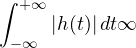
Theorem. An LTI system is BIBO stable if and only if its impulse response is absolutely integrable:
Proof. *Sufficiency:* if  for every , then

which is finite. *Necessity:* if the integral diverges, choose the bounded input  ; at
 the output equals
 . ∎
The RC circuit is stable ( ); an ideal integrator, with
 , is not: a step at the input produces a ramp that grows without bound.