ACC 2: sensors and configurations, camera only, camera and radar, several radars
1V, 1R1V and 5R1V configurations, camera distance proved with its quadratic error, time to collision from scale, FMCW radar, radar lateral error, hard cases and stationary objects.
https://www.electronics-engineering.com/en/acc-sensors-camera-radar-configurations-measurement-errors/
An ACC is as good as what it sees. Following a vehicle requires three numbers: the distance  , the relative speed
 and the lateral position
 , which says whether the vehicle is in our lane. Camera and radar measure these numbers in very different ways, with errors that grow with distance in different ways: this is why configurations with several sensors are not only about seeing further, but about covering the weak points of each one. In this lesson we derive the measurement errors from geometry and physics, and we will use them in the next one for fusion.
The configurations
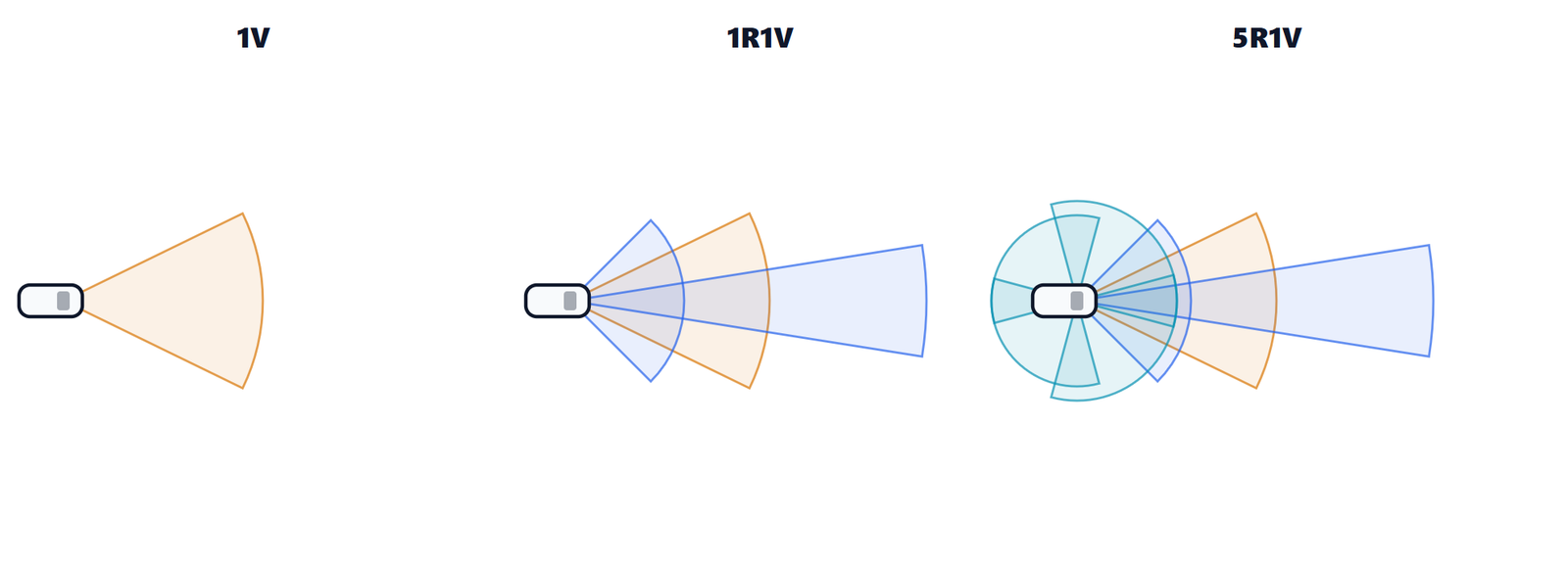
| Configuration | Sensors | Strengths | Limits |
|---|---|---|---|
| 1V | one camera | cost, classifies objects, sees the lines | imprecise distance far away, blind with low sun, fog, darkness |
| 1R1V | front radar + camera | precise distance and speed, works in rain and darkness | radar angle less precise, ambiguous stationary objects |
| 1V3R, 1V5R | + corner radars | sees vehicles entering the lane (cut-ins) earlier, lane change | more data to fuse and calibrate |
| nV nR (+ lidar) | cameras around the car, several radars | 360° view, redundancy | computation, cost, complexity |
1R1V is the most common case in series production cars: radar and camera complement each other. “Vision only” solutions use several cameras and neural networks that estimate distance; they are feasible, but distance accuracy remains the weak point, as the numbers will show.
The camera: distance from the road plane
A camera sees an image, not a distance. The most common way to get it with a single camera is the point where the vehicle touches the road.
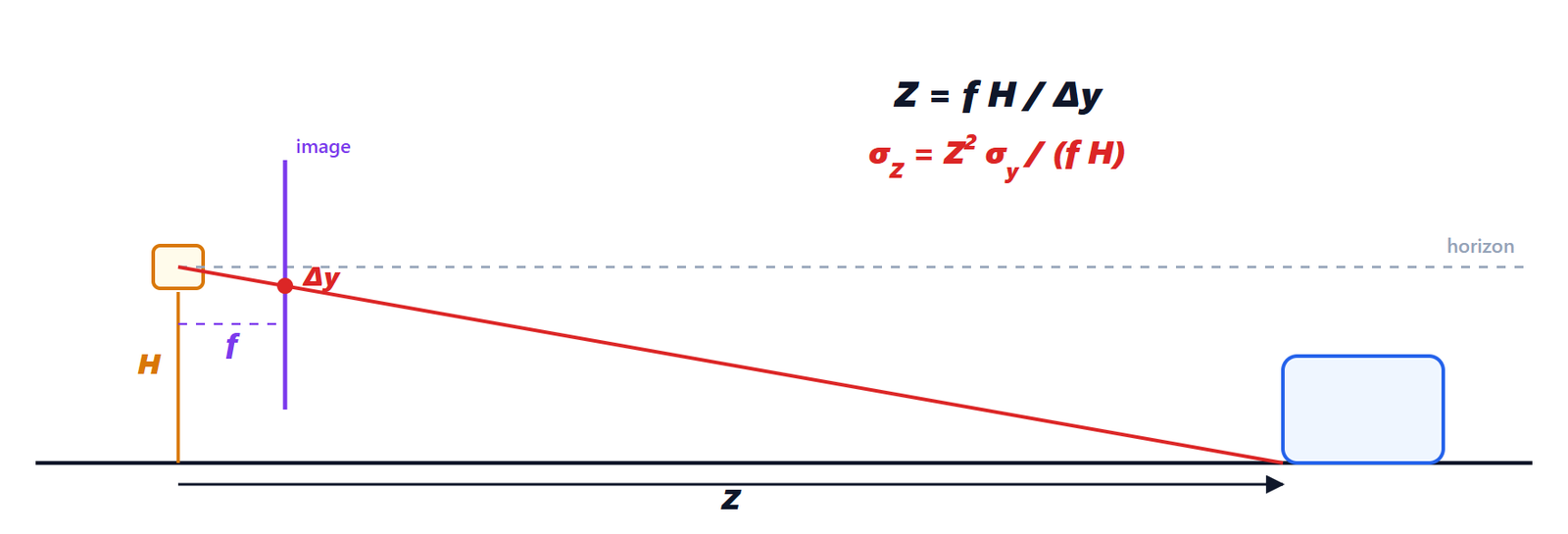
 above the road, with focal length
 (in pixels). The point where the wheels of the vehicle touch the road, at distance
 , appears in the image
 pixels below the horizon. The two similar triangles give
 .
Proof. The ray from the camera to the contact point drops by over a distance ; on the image plane, at distance from the optical centre, the same ray drops by . The two triangles are similar, so  , that is

Now the error. If the contact point is estimated with an error of  pixels, the distance error is the derivative times the error (first-order propagation):

The error grows with the square of the distance. With  px,
 m and one pixel of error: 1.6 m at 50 m, 6.4 m at 100 m, 14 m at 150 m. At 100 m the camera cannot tell whether the vehicle is at 94 or 106 m, let alone how fast it is approaching: differentiating such a noisy distance gives an unusable relative speed. Moreover, the formula only holds on a flat road: a slope or the pitch of the car under braking (one degree of pitch moves the horizon by 21 pixels) distort .
There is a second way, the apparent width: a car of width  appears
 pixels wide. But is unknown (a small car is 1.6 m, a truck 2.5 m): a 10% error on is a 10% error on the distance.
Time to collision without knowing the distance
The camera, however, has a weapon the radar does not have. Differentiating with respect to time:

The ratio between the width in the image and its growth rate is the time to collision (TTC), and it depends neither on nor on . Camera-only emergency braking functions use exactly this: for safety what matters is how much time is left, not how many metres.
The lateral position, instead, the camera measures well: an object at column  from the image centre is at
 , with an error of about
 : 12 cm at 100 m. The camera also sees the lane lines, which we will need in lesson 4 to predict where our car will go.
The FMCW radar
The 77 GHz automotive radar transmits frequency ramps (chirps) and compares the echo with the transmitted signal. We saw how it works in detail in the lesson on the FMCW automotive radar; here we need three formulas and where they come from.
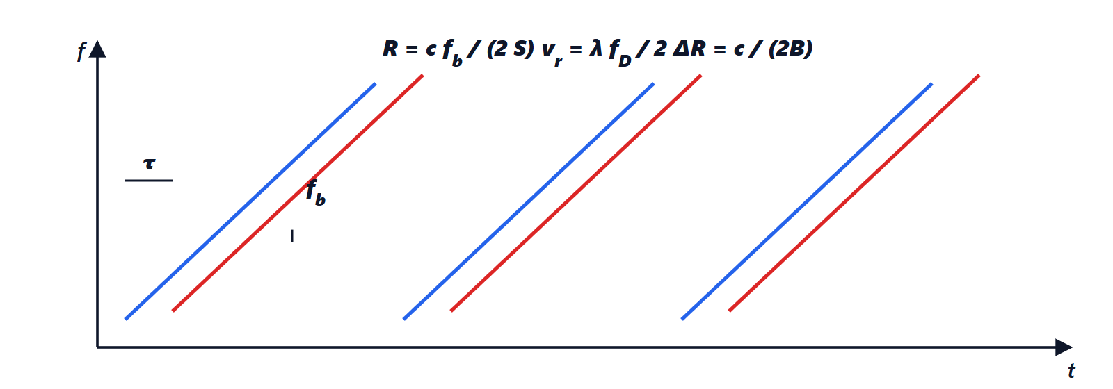
 , so at every instant the two frequencies differ by the beat frequency
 , with
 the slope of the ramp. The motion of the target adds the Doppler shift
 .
- range:
 , so
 . The resolution (the smallest range difference between two separable targets) is
 , with
 the frequency sweep: with
 GHz, 15 cm;
- radial speed: the echo of a target moving at speed
 is shifted by
 ; at 77 GHz
 mm. The radar measures the relative speed directly, without differentiating the distance, with errors of a few cm/s;
- angle: with several receiving antennas (and several transmitting ones, MIMO) the phase difference between two antennas at distance
 is
 . Typical accuracy is a few tenths of a degree.
The weak point is precisely the angle: an error  becomes a lateral error

which grows linearly with distance: with 0.3° (0.0052 rad), 0.26 m at 50 m, 0.52 m at 100 m, 0.79 m at 150 m. A lane is 3.5 m wide: at 150 m the radar struggles to tell which lane a vehicle is in.
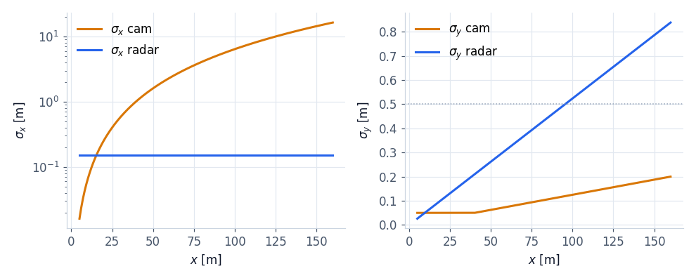
The chart is the reason for the 1R1V configuration: the radar is precise where the camera is weak (distance, relative speed) and the camera is precise where the radar is weak (lateral position). Lesson 3 will show that the Kalman filter automatically takes the best of each.
The hard cases
| Situation | Camera | Radar |
|---|---|---|
| low sun, glare, darkness | degrades or blind | not affected |
| heavy rain, fog, snow | degrades a lot | degrades a little (spray, snow on the sensor) |
| stopped vehicle in the lane | recognises it as a vehicle | echo identical to manhole covers, signs, bridges: all stationary |
| tunnel, guard rail | lines often visible | multiple reflections, ghost targets |
| very close vehicle cutting in | often outside the field of view | narrow beam: sees it late, corner radars needed |
| unusual vehicles (trailers, oversized loads) | classification can be wrong | sees them, shape uncertain |
The most important case for ACC is the stopped vehicle. For the radar every stationary object approaches at the speed  of our car: a car stopped in a queue, a manhole cover, the structure of a bridge and a sign all have the same relative speed. Without other information, braking for every stationary echo means braking for nothing (false positive), ignoring them all means not stopping behind a queue. The solutions we will see in lesson 4 are camera confirmation and the memory of objects seen moving. Newer radars (called 4D or imaging) also measure elevation and tell a bridge from a car better, but the problem remains.
What the sensor must give to fusion
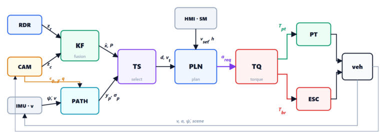
Every sensor sends to the ADAS ECU, every cycle, a list of objects with measurements and uncertainties. In the code:
def radar_measure(prm, rng, x, y, vx):
    """Polar measurement of a target at (x, y): (range, azimuth, range rate) or None."""
    r, th = sqrt(x * x + y * y), atan2(y, x)
    if r > prm.r_max or abs(th) > prm.fov or rng.random() > prm.p_det:
        return None                          # out of the beam or missed detection
    rr = vx * cos(th)
    return (r + rng.normal(0, prm.sigma_r), th + rng.normal(0, prm.sigma_th), rr + rng.normal(0, prm.sigma_rr))


def camera_sigmas(prm, x):
    """sigma_x = x^2 / (f h) sigma_px (ground plane), sigma_y ~ x / f sigma_px"""
    return x * x / (prm.f * prm.h) * prm.sigma_px, max(0.05, x / prm.f * prm.sigma_px * 1.5)
Uncertainties are not a detail: the Kalman filter weights every measurement with the inverse of its variance, and a sensor that declares too small an error takes over even when it is wrong. In the next lesson we build the tracker that merges the two lists into a single list of reliable objects.