ACC 4: target selection, path prediction and false positives
Path from yaw rate and lane lines fused with their uncertainty, in-path probability proved, false positives in curves, stationary objects, state machine, predicted cut-in.
https://www.electronics-engineering.com/en/acc-target-selection-path-prediction-cut-in-false-positives/
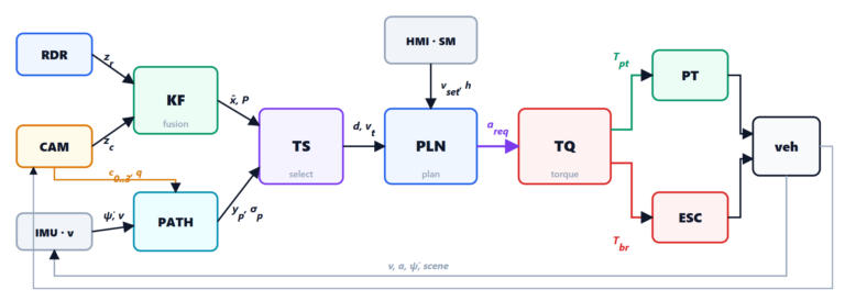
Fusion gives a list of objects: cars in our lane, cars in the neighbouring lanes, guard rails, signs, sometimes a ghost echo. Target selection chooses which one to follow. There are two possible mistakes and they weigh differently: a false positive (braking for a car that is in the next lane) is annoying and dangerous, because whoever follows does not expect it; a false negative (not seeing in time a car that enters our lane) forces hard braking at the last moment. The heart of the problem is predicting where our own car will go, even when the lines on the road are poorly visible.
Where we will go: the predicted path
From the yaw rate
A car driving through a curve of radius  at speed
 rotates with angular velocity
 , so the curvature is
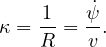
The gyroscope measures  always, in any weather. If the curvature stays as it is now, the path is a circle: the point at distance
 ahead is at lateral position
 . For
 , with the expansion
 :

But the curvature changes. Roads are built with transition curves whose curvature varies linearly with distance (clothoids),  . The heading angle is
 and, integrating again, the lateral displacement is
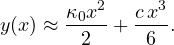
The gyroscope sees  but not
 : at the entry of a curve our car still drives straight while the road already turns, and the error grows with
 . In the model we treat as uncertain (standard deviation
 m⁻², typical of motorway transition curves) and the gyroscope noise as uncertainty on : the uncertainty of the path grows quickly with distance.
From the lane lines
The camera gives the centre of the lane as a polynomial  , with a quality
 (contrast, both lines visible, line type) and a view range (how far the lines are seen). The lines “see” the curve before we enter it, but they can be missing: road works, snow, worn lines, junctions. Their error grows with distance and becomes huge beyond the view range.
Fusing the two paths
Each point has two estimates with their standard deviations,  and
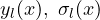 . They are combined like two independent measurements (the same proof as in lesson 3): weights inversely proportional to the variances,
 . With good lines the camera wins; with poor lines the yaw rate remains, with an uncertainty that honestly says how little we know.
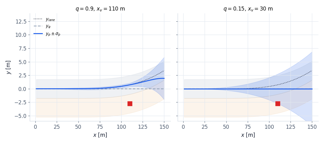
 , view range 110 m): the fused path (blue, with the band
 ) follows the curve, at 110 m 0.73 ± 0.33 m against a true 0.74. Right, poor lines (
 , 30 m): the path stays straight but the band widens, ±2.7 m at 110 m. The red square is a car in the right lane.
The probability of being on our path
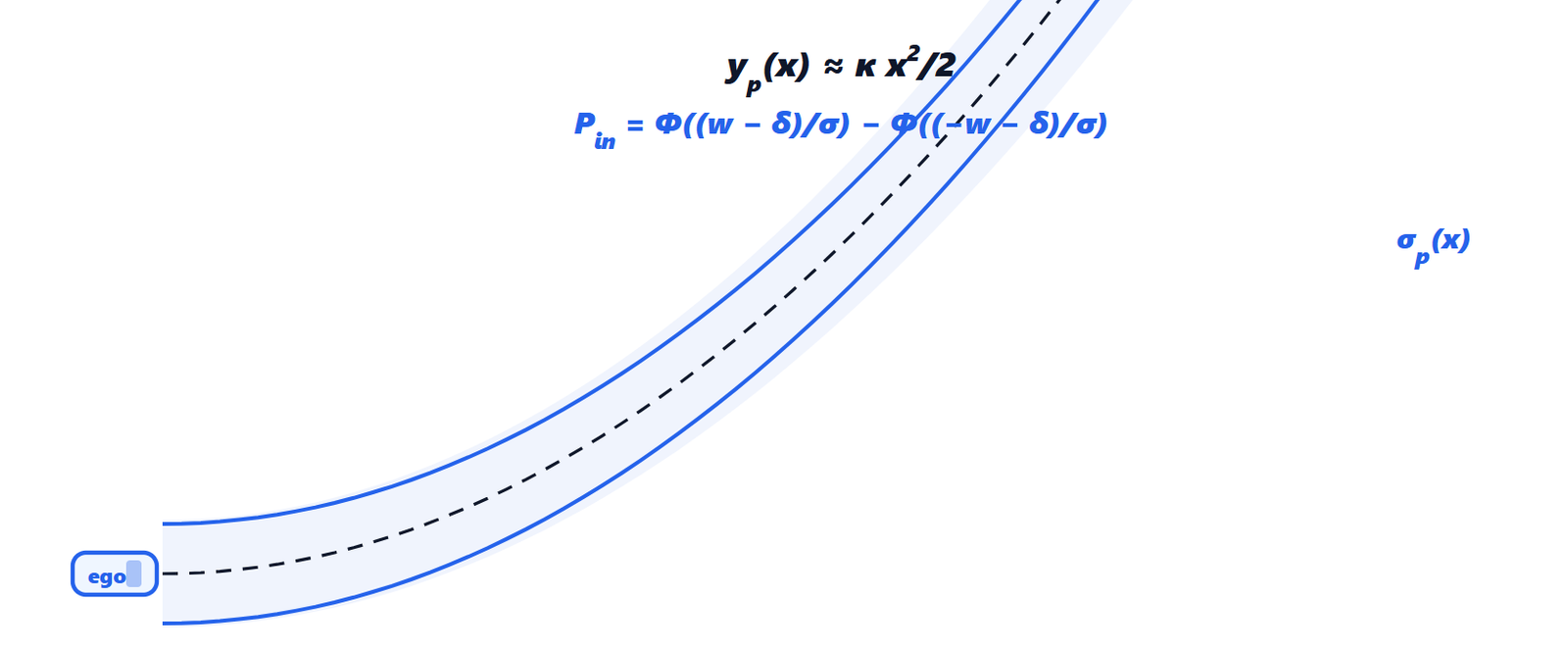
 around the predicted path
 and an object with lateral offset
 . The light blue band represents the uncertainty
 , which grows with distance.
For an object at distance and lateral position  , the offset from the path is
 . The true offset is uncertain: adding the uncertainty of the object (from the tracker covariance) and that of the path,
 . The object is on our path if the true offset lies within the corridor
 ; with a Gaussian offset of mean , the probability is the integral of the Gaussian between
 and :

with  the cumulative distribution function of the standard normal. The half width
 m is that of our car plus a margin, not that of the lane: what matters is whether the other vehicle occupies the space we will sweep, not where the lines are.
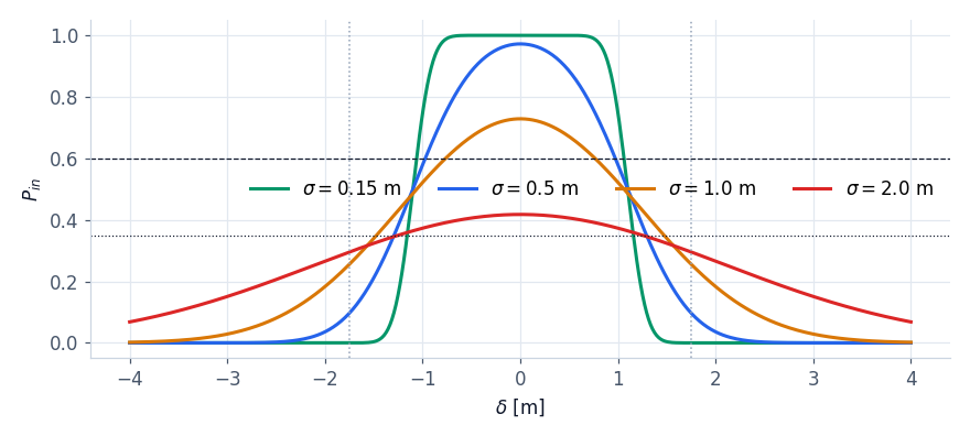
 as a function of the offset for different total uncertainties. With
 m the curve is almost a rectangle: in or out. With
 m it does not exceed 0.4 even at the centre: a distant object with an uncertain path cannot become the target. The horizontal lines are the entry (0.6) and exit (0.35) thresholds.
This is already a defence against false positives: where we do not know where we will go, no object exceeds the threshold.
False positives and how to avoid them
The classic case: we approach a left curve; a car in the right lane, 95 m ahead, is already in the curve. Relative to our current, straight direction, its displacement brings it right in front of us: a selector that uses only the yaw rate with a fixed uncertainty takes it as the target and brakes.
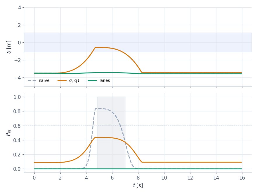 . With the naive selector (path from the yaw rate only, fixed uncertainty, grey) the probability reaches 0.84 and the car is taken as the target for 2.2 s (shaded area): braking for nothing. With poor lines but honest uncertainty (orange) it reaches 0.44: never a target. With good lines (green) it stays at 0.
The defences, all in the code:
- path with honest uncertainty: the uncertainty grows with
 and ; with poor lines a distant object does not reach the threshold;
- no new targets where the path is too uncertain: if
 m at the object’s distance, the object cannot become a candidate (a target already locked is kept, with hysteresis);
- confirmation time that grows with uncertainty: a candidate must stay above the threshold for
 seconds;
- hysteresis: entry with
 , exit with
 : no target that appears and disappears;
- stationary objects: for the radar they are all the same (lesson 2). A stationary object is admitted only if it has been seen moving (a car that stopped in a queue) or if the camera has confirmed it within the last 0.5 s and it is within 80 m;
- confirmed tracks only: isolated echoes never get here (M-of-N logic of lesson 3).
The selection state machine
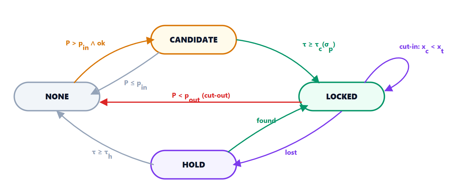
 ; it must stay there for
 . LOCKED: it is the target the planner follows; if a closer object becomes a confirmed candidate it replaces it (cut-in); if falls below
 it is released (cut-out). HOLD: the target track was lost for a moment; its prediction is kept for
 , then NONE.
| From | To | Condition |
|---|---|---|
| NONE | CANDIDATE | closest admitted object with and  m |
| CANDIDATE | NONE | the candidate drops below 0.6 or disappears |
| CANDIDATE | LOCKED | it stays above the threshold for s |
| LOCKED | LOCKED (new) | a closer object is a candidate for  : cut-in |
| LOCKED | NONE | or object no longer admitted: cut-out |
| LOCKED | HOLD | the target track is missing (lost measurements, occlusion) |
| HOLD | LOCKED | the track comes back |
| HOLD | NONE | 0.6 s have passed |
The HOLD state looks like a detail, but without it every time the radar loses the target for a few cycles (it happens, for example, under a bridge) the ACC would accelerate towards the set speed and then brake again. In lesson 7 a 0.4 s loss of radar measurements passes without a single cycle without a target.
The cut-in: predicting who comes in
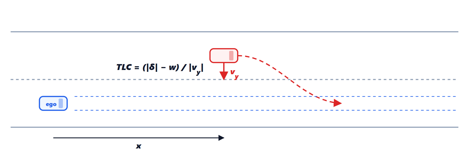
 . The time to line crossing, TLC, is the offset still to cover divided by the lateral speed.
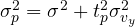
Waiting until the car is already in the corridor means reacting late. If an object outside the corridor is moving towards it, we also compute where it will be in  s,
 , with an uncertainty increased by the variance of the lateral speed (
 ), and we use the higher of the current and the predicted probability (the latter multiplied by 0.9: a prediction is worth a little less than a measurement).
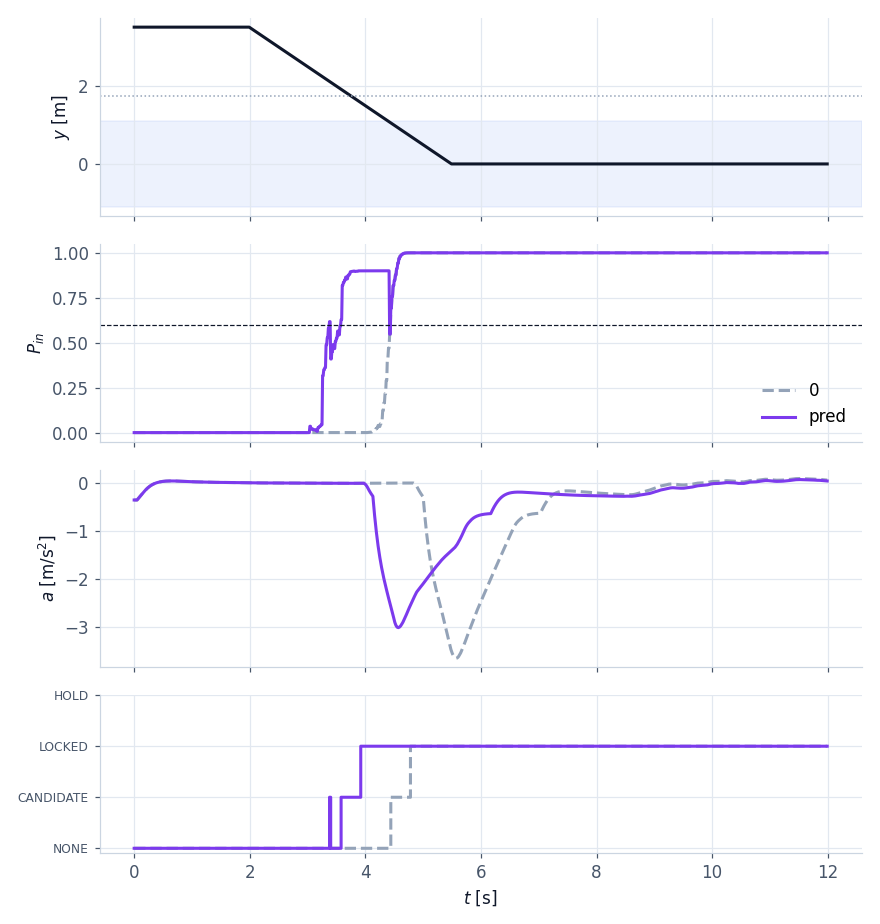 , acceleration of our car, selection state. With prediction (violet) the target is locked at 3.92 s, when the car is still 1.57 m from the centre; without (grey) at 4.78 s. Result: peak braking 3.0 m/s² instead of 3.7, minimum distance 34.0 m instead of 31.5.
The code
Here is the evaluation of an object in the C version (the Python one is identical):
static bool ts_assess(TgtSel *s, const AccObject *o, const AccPath *path, float v_ego, float t, float *prob, float *sp)
{
    float yp, sig, delta, v_abs;
    bool stationary, ok;
    *prob = 0.0f; *sp = 0.0f;
    if (o->x <= 0.5f) return false;
    PathPred_At(path, o->x, &yp, sp);                 /* fused path and its sigma at the object */
    delta = o->y - yp;
    sig = sqrtf(o->var_y + *sp * *sp);
    *prob = InPathProbability(delta, sig, TS_HALF);
    if (fabsf(o->vy) > 0.2f && sgnf(o->vy) == -sgnf(delta) && fabsf(delta) > TS_HALF) {
        float d_pred = delta + o->vy * TS_T_PRED;      /* cut-in: where it will be */
        float s_pred = sqrtf(sig * sig + TS_T_PRED * TS_T_PRED * o->var_vy);
        *prob = maxf(*prob, 0.9f * InPathProbability(d_pred, s_pred, TS_HALF));
    }
    v_abs = v_ego + o->vx;
    stationary = fabsf(v_abs) < 1.0f && !was_moving(s, o->id, fabsf(v_abs) > 3.0f);
    ok = o->confirmed;
    if (stationary)       /* stationary: camera confirmation and close range */
        ok = ok && (t - o->t_cam < 0.5f) && o->x < TS_X_STAT;
    return ok;
}
Now we know which vehicle to follow, its distance  , its speed
 and its acceleration
 . In the next lesson we decide how to follow it: how much to accelerate or brake, cycle after cycle.