ACC 5: planning, following, elastic approach, preboost and stop & go
Short, middle, long and extra long time gaps, stability and string stability proved, kinematic approach with elasticity, overtaking preboost, stop & go stopping law, MPC.
https://www.electronics-engineering.com/en/acc-planning-time-gap-string-stability-approach-preboost-stop-and-go/
We have the target: its distance  , its speed
 , its acceleration
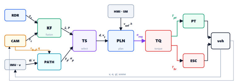
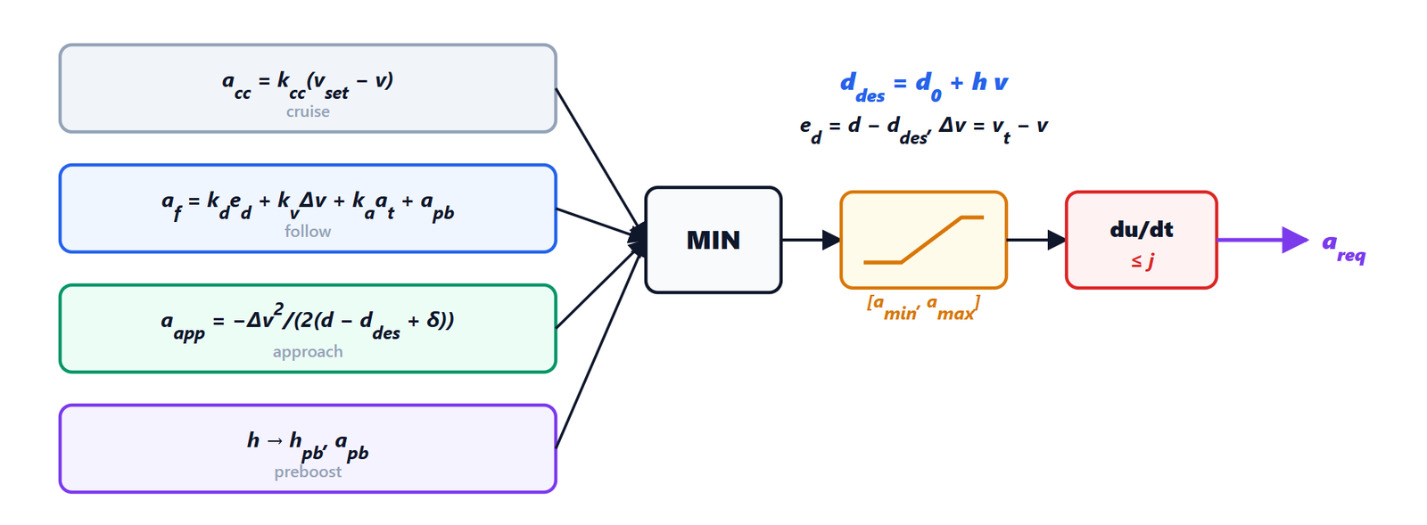
 . Every 20 ms the planner decides which acceleration to request from the car. A single controller is not enough: following in steady state, approaching a much slower vehicle, preparing an overtake and stopping in a queue are different problems with different solutions. The structure we use is that of many series systems, rule-based: each mode proposes an acceleration, the most cautious one wins, then limits and jerk.
 to torque control.
The constant time gap policy
The desired distance is  : it grows with our speed. The errors the planner uses are

Why this and not a fixed distance? With a fixed distance a string of cars with ACC amplifies disturbances along the string unless the vehicles communicate; with a time gap this can be avoided, as we prove shortly. The driver chooses  among four values.
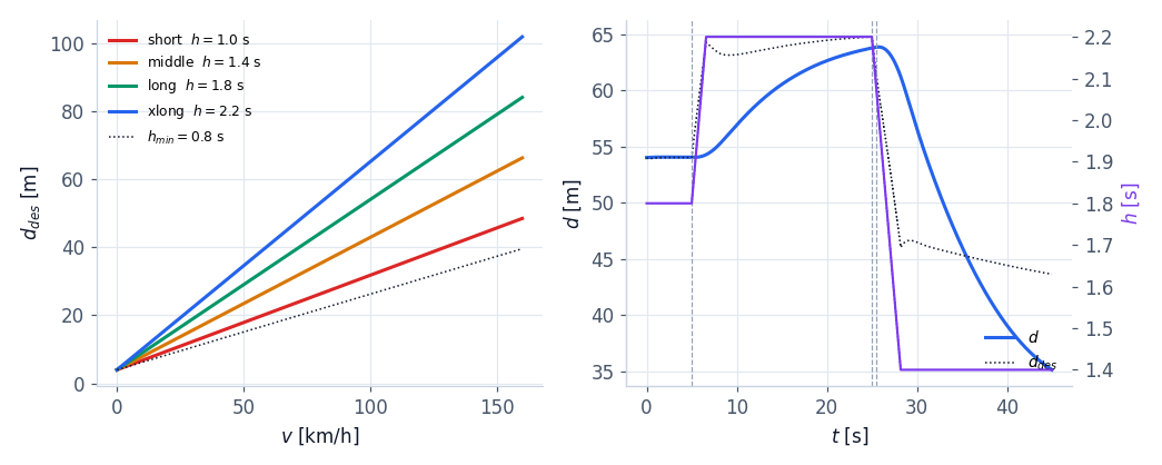 (violet) changes by 0.25 s per second and the distance follows it without jerks.
The change of is deliberately slow: a jump from 2.2 to 1.0 s would mean a distance error of 33 m in an instant, and the controller would accelerate all at once.
Steady-state following
The basic mode is a proportional-derivative controller on the distance error, with the target acceleration fed forward:

Stability. Let us assume for now that the car achieves the requested acceleration immediately ( ) and that the target drives at constant speed. Then
 and
 , that is

The trace is  , the determinant
 : the characteristic polynomial is

stable for every  ,
 (the Routh criterion for second order). With
 s: natural frequency
 rad/s and damping
 , that is no overshoot (the second-order response). A slow, calm following is what is wanted: nobody wants a car that reacts to every small change of the vehicle ahead.
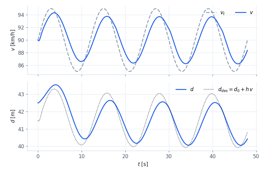
String stability
A single stable car is not enough. In a string of cars with ACC each one follows the previous one: if each amplifies the speed variations a little, the last one suffers a huge disturbance (it is the wave that appears out of nowhere in traffic jams). With Laplace transforms (see transfer functions), for car  following car
 :

The string does not amplify disturbances if  at every frequency. With
 :

The worst case is  ; dividing by
 gives the condition

With  ,
 : for
 it is 2.14 and fine; for
 it is 1.35 and the string amplifies. This is why the gains cannot be fixed: in the code
 grows when the time gap gets shorter,
 , that is 0.98 for s.
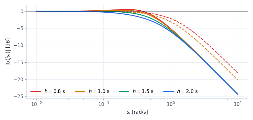
 in decibels for different time gaps with fixed gains (solid lines): for 0.8 and 1.0 s it exceeds 0 dB, the string amplifies. The dashed lines are the same time gaps with adapted: they stay below 0 dB.
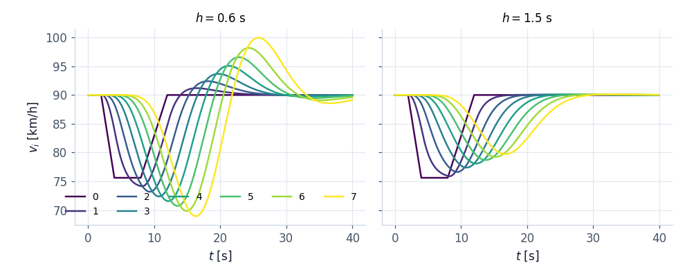
 s and fixed gains (left) the wave grows: the first drops to 75.6 km/h, the last to 68.9. With s (right) it is damped: the last drops only to 79.7 km/h. The actuators have a delay of 0.2 s, which worsens the condition: it is one of the reasons for the 0.8 s minimum of the standard.
Approaching a slower vehicle
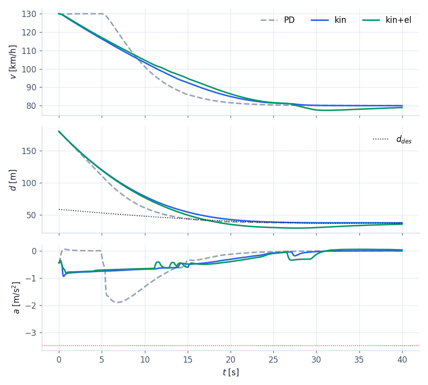
We arrive at 130 km/h and ahead, at 200 m, there is a car at 80 km/h. The following controller, left alone, waits until the distance error becomes small and then brakes hard: with  m/s the term
 is
 m/s², limited to
 . An experienced driver does something else: stops accelerating, then brakes gently and steadily.
The kinematic deceleration. In relative motion, with the target at constant speed, a constant deceleration  cancels the speed difference
 after a relative distance
 given by
 . If we want to vanish exactly when the distance reaches
 , we need
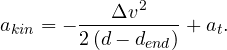
Recomputed every cycle, this law corrects its own errors: if the car brakes less than planned, the remaining distance shrinks and the request grows.
Elasticity. It is not necessary to arrive exactly at  with
 . If we accept going temporarily below the desired distance by a margin
 and recovering it calmly afterwards, the distance available for braking grows and the braking gets softer: with
 ,

In the code  : a quarter of the desired distance, never more than 12 m.
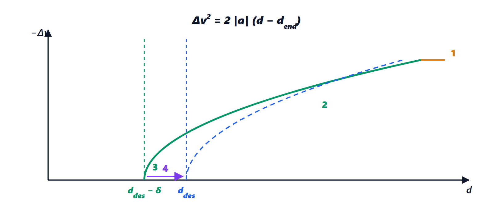
 , which ends at
 instead of (dashed); (3) a short elastic undershoot; (4) gentle recovery to .
Three details make the manoeuvre robust:
- mode with hysteresis: the approach starts with a real closing speed (above 1 m/s) and ends when it is almost zero or the elastic margin is used up; without hysteresis, with close to zero the mode switches on and off;
- mild phase: as long as
 is weaker than what releasing the pedal gives (
 m/s²), the following controller does the job, but without braking more than necessary (
 ) and without closing faster than
 ;
- elastic recovery: after the approach the missing distance is recovered with a reduced gain (
 ) and a deceleration of at most
 m/s²: the distance opens up because we slow down slightly, not because we brake.
Overtaking preboost
We follow a truck at 80 km/h with the set speed at 130. The driver signals left to overtake. A simple ACC keeps the 37 m of distance until the truck has left the corridor, and only then accelerates: the overtake starts slowly, and whoever comes from behind in the overtaking lane has to brake.
Preboost anticipates the overtake: with the indicator towards the overtaking lane, a target slower than the set speed and the next lane free (corner radars and fusion say so), the planner
- reduces the time gap towards
 s, always with the slow change of 0.25 s per second;
- adds an acceleration
 m/s² to the following term;
- stops after 4 s if the lane change does not happen, or as soon as the indicator is switched off, and the distance goes back gently to its normal value.
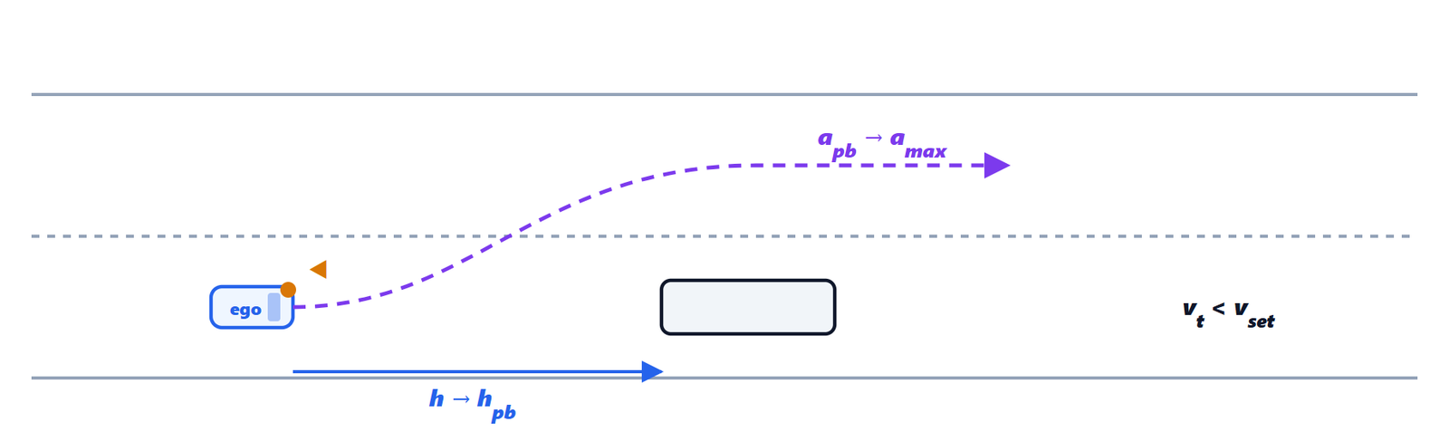
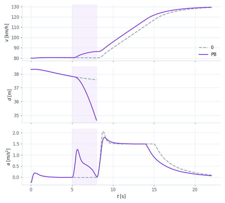
 and the car starts accelerating before the truck has left the corridor; after the lane change the target is free and the acceleration rises towards
 .
Stop & go
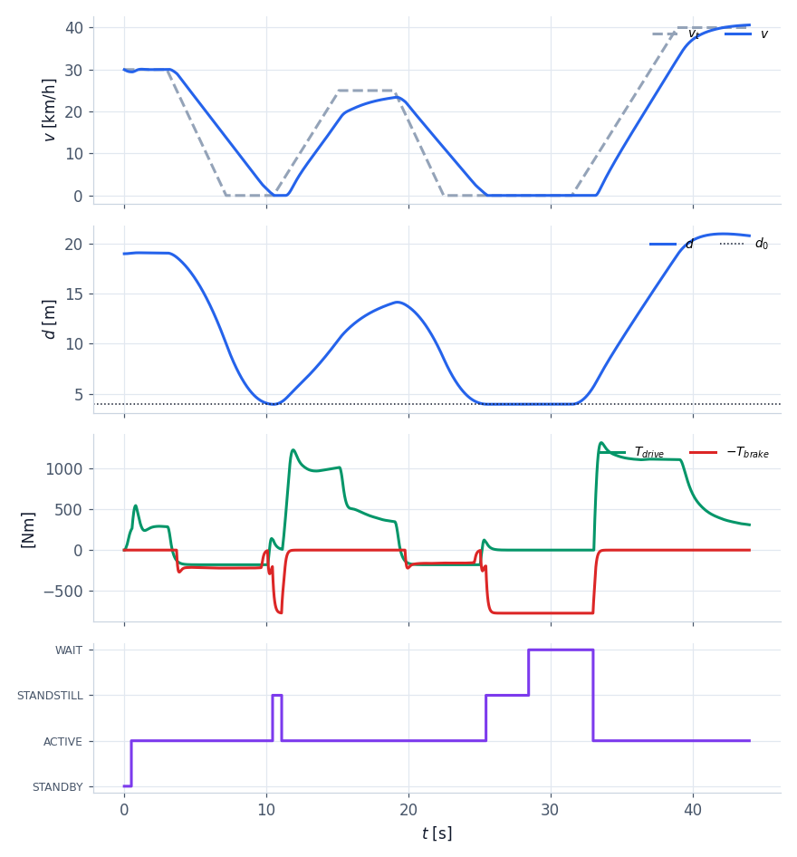
In a queue the target brakes until it stops. The following controller, with the target acceleration fed forward, would copy its braking and stop us where we are, perhaps at 15 m. What we need is to stop  from the point where the other one will stop.
The stopping law. If the target brakes with  , it will stop after the distance
 , that is at the distance
 from us. To stop behind that point with constant deceleration:
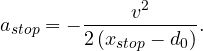
If the target is already stopped,  . The law replaces following and approach when the target will stop within 4 s and we are below 54 km/h. At low speed the wider limits of ISO 22179 apply, interpolated as seen in lesson 1: down to −5 m/s² and up to +4 m/s² below 18 km/h. When we are stopped less than
 m from the stopped target, the planner requests the stop and the state machine goes to STANDSTILL: the brakes hold the car (lesson 6).
Arbitration, limits and jerk
The proposals of the modes (set speed  , following, approach, stop) go into the minimum block: the most cautious wins. Then:
- saturation to the limits of the standard, which depend on speed (from /
 m/s² above 72 km/h to
 /
 below 18 km/h);
- jerk limit: the request changes by at most 2.5 m/s³ (comfort); in firm braking (below
 m/s²) up to 5 m/s³ at low speed.
self.mode = min(cands, key=cands.get)                  # the most cautious proposal wins
a_lo, a_hi, j_lo = iso_limits(v, p)                    # ISO 15622 / 22179, speed dependent
a_goal = float(np.clip(cands[self.mode], a_lo, a_hi))
if self.stop_request:
    a_goal, self.mode = min(a_goal, -0.5), "stop"
jerk = j_lo if a_goal < -2.0 else p.jerk_max
self.a_out += float(np.clip(a_goal - self.a_out, -jerk * dt, p.jerk_max * dt))
The alternative: model predictive control
A different approach is model predictive control (MPC), which we saw in the lesson on optimal and predictive control. With the state  and the model of relative motion, every cycle a quadratic problem is solved over a horizon of a few seconds: minimise a weighted sum of distance error, speed difference, acceleration and jerk, with explicit constraints (limits of the standard, minimum distance, set speed). Gentle approach, elasticity and early braking come out of the cost and the constraints by themselves.
| Rule-based (this lesson) | Predictive (MPC) | |
|---|---|---|
| behaviour | designed mode by mode | comes from cost and constraints |
| constraints | with saturations and special cases | explicit, met by construction |
| computation | microseconds | a quadratic problem every 20 ms |
| calibration and certification | every parameter has a physical meaning | less intuitive weights, solver to qualify |
Many series systems stay rule-based precisely because of the last row; MPC is used more and more where the ECU has computing power and long predictions are needed (curves, speed limits, lane changes).
The request is ready. But the car has no acceleration command: it has an engine and brakes. In the next lesson we turn it into wheel torque, with all the physics of the vehicle.