Time response: first and second order, overshoot and dominant poles
Poles and zeros, step response of first- and second-order systems, overshoot with proof, settling and rise time, specifications in the s-plane, dominant poles.
Control system specifications are often given in time: “the temperature must reach the requested value in less than two minutes, without exceeding it by more than 5%”. To translate them into design conditions you need to know how pole locations determine the shape of the response. In this lesson we cover the step response of first- and second-order systems, the formulas for overshoot and settling time, and the idea of dominant poles.
Poles and zeros
A rational transfer function  has zeros (roots of the numerator) and poles (roots of the denominator). Expanding in partial fractions, the response to any input contains a term
 for each pole
 : real if the pole is real, oscillating if it is complex. The location of the poles in the complex plane therefore decides the shape of the response.
First order
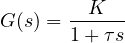
has a pole at  . The unit step response is

After a time  the output is at 63% of its final value, after
 at 95%, after
 at 98%. The further the pole is from the imaginary axis, the faster the response. Many thermal processes and the motor with negligible inductance behave this way.
Second order
The standard form is
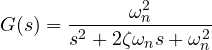
with natural frequency  and damping ratio
 . For
 the poles are complex conjugate:

In the complex plane they lie at distance from the origin, and the angle  they make with the negative real axis satisfies
 .
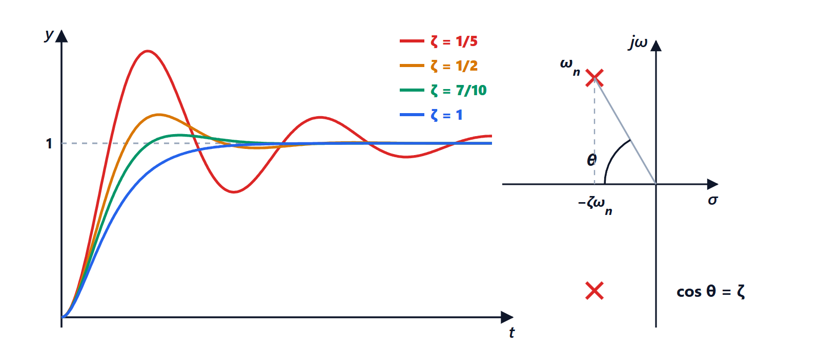
The unit step response is

an oscillation at angular frequency  inside an envelope decaying as
 .
Time-domain specifications
Theorem (overshoot). The peak of the response occurs at  and the overshoot is

Proof. The derivative of the step response is the impulse response,  , which first vanishes (after
 ) at
 . There
 , so
 , and
 . ∎
Overshoot depends only on the damping ratio:
| 0.2 | 0.4 | 0.5 | 0.6 | 0.7 | 0.8 | 1 |
|---|---|---|---|---|---|---|---|
 | 52.7% | 25.4% | 16.3% | 9.5% | 4.6% | 1.5% | 0 |
A value of around 0.7 is a classic compromise: a fast response with less than 5% overshoot.
Settling time. The envelope drops below 2% for  :

It depends only on the real part of the poles: to settle faster the poles must lie further to the left.
Rise time. The time to go from 10% to 90% is, for around 0.5, about  : it depends mainly on the distance of the poles from the origin.
Specifications thus become regions of the s-plane: a maximum overshoot means poles inside a sector of maximum angle ; a maximum settling time means poles to the left of a vertical line. Design consists of bringing the closed-loop poles into that region.
Dominant poles
Real systems have many poles, but poles far from the imaginary axis produce terms that die out quickly. If one pair of poles is much closer to the axis than the others (at least five times), the response is nearly that of a second-order system with only those poles, the dominant poles. That is why second-order formulas are used everywhere as a first approximation.
Zeros modify the response: a left-half-plane zero close to the dominant poles increases overshoot; a right-half-plane zero (“non-minimum-phase” systems) produces a response that starts off in the wrong direction, like the altitude of an aircraft which, when the elevator is raised, dips for a moment before climbing.