Control systems: feedback, sensitivity and models
Open and closed loop, loop transfer functions with proof, sensitivity and disturbance rejection, the DC motor model, linearisation.
A control system makes a physical quantity follow a desired value: the temperature of an oven, the speed of a motor, the altitude of a drone, the output voltage of a power supply. The key idea is feedback: continuously measure the result and correct the action according to the error. In this lesson we see why feedback works, how the transfer functions of a loop are written and how a model of a physical system is built.
Open loop and closed loop
In open loop the command is computed in advance: a toaster heats for a fixed time, without knowing whether the bread is ready. It works only if the system model is exact and there are no disturbances.
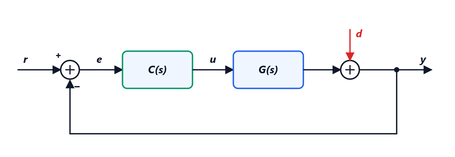
In closed loop a sensor measures the output  , it is compared with the reference
 , and the controller
 decides the command
 based on the error
 . The plant
 is the system to be controlled, and
 represents the disturbances acting on the output.
The loop transfer functions
Theorem. With the notation of the diagram and  (the loop function),

Proof. From the diagram  ,
 ,
 . Substituting,
 , that is
 . ∎
The two functions have names:

and  . If the loop gain
 is large,
 (the output follows the reference) and
 (the disturbance is almost removed).
Why feedback works
Disturbance rejection. A disturbance that in open loop would reach the output in full is reduced  times.
Insensitivity to plant variations. The real plant is never identical to the model: components age, the load changes.
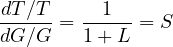
Theorem. The relative change of  due to a relative change of
 is reduced by the factor
 :
Proof.  , so
 . Multiplying by
 gives
 . ∎
With a loop gain of 100, a 10% error in the plant becomes a 0.1% error in the closed-loop behaviour. It is the same principle as feedback operational amplifiers, whose gain depends only on two resistors and not on the transistor.
The price. Feedback can make a stable system unstable (corrections that are too strong and too late make the loop oscillate), and it brings sensor noise to the output, with transfer function  . The next lessons are about handling these two problems.
Models of physical systems
Designing the controller requires a model of the plant. The physical equations are written, usually differential equations, and their Laplace transform is taken with zero initial conditions (Mathematical Methods lessons).
Example: the DC motor. The armature circuit has resistance  and inductance
 ; the motor generates a back EMF
 and a torque
 (the same constant
 for both, in SI units); the rotor has inertia
 and viscous friction
 :

Transforming and eliminating  :

a second-order system. With negligible inductance it becomes first order,  , with a single mechanical time constant.
Linearisation
Many systems are not linear: a pendulum has the equation  . The methods of this course apply to linear systems, and are used by linearising around an equilibrium point with a first-order Taylor expansion (Analysis 1 lesson): near
 ,
 , and the equation becomes linear. A controller designed on the linearised model works as long as the system stays close to equilibrium, and feedback itself helps keep it there.





