Computer architecture: the von Neumann model, performance and Amdahl's law
CPU, memory and bus, the Harvard architecture, the instruction cycle, the performance equation with an example, Amdahl's law with proof and examples.
A computer, from the microcontroller in a washing machine to a server processor, executes a sequence of instructions taken from memory. The basic organisation is still the one proposed by von Neumann in 1945; what has changed enormously is how it is built to go fast. In this lesson we cover the von Neumann model, the instruction cycle, how performance is measured and Amdahl’s law, which says how much can be gained from an improvement.
The von Neumann model
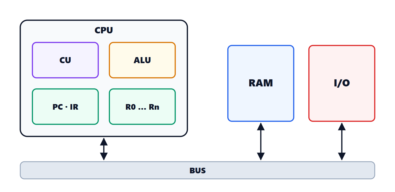
- The CPU contains the control unit (CU), which interprets instructions and drives everything else; the arithmetic logic unit (ALU), which does the calculations; the registers, tiny very fast memories. Two special registers: the program counter (PC) with the address of the next instruction and the instruction register (IR) with the one being executed.
- The main memory holds both data and instructions: this is the stored-program idea, which makes the computer universal (changing task means loading another program, not rewiring the machine).
- The input and output (I/O) devices and the bus connecting everything.
In the Harvard architecture instructions and data live in separate memories, with two buses: an instruction and a data item can be read at the same time. Many microcontrollers and signal processors use it; modern processors are von Neumann towards main memory, but have separate caches for instructions and data.
The instruction cycle
The CPU repeats forever:
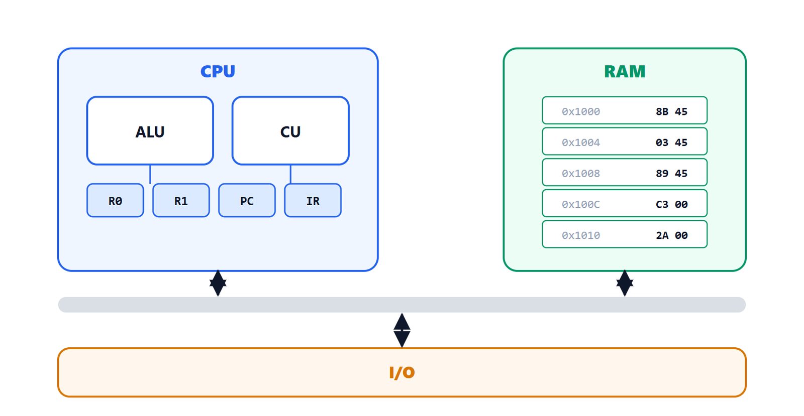
- fetch: read from memory the instruction at the address held in the PC and place it in the IR; the PC moves on to the next instruction;
- decode: the control unit works out which instruction it is and reads the operands from the registers;
- execute: the ALU computes, or memory is read or written;
- write back the result into a register.
A jump modifies the PC, and the next fetch continues from another point of the program: this is how loops, conditions and function calls are implemented. Everything is paced by a clock, a periodic signal whose frequency (a few gigahertz today) sets the rhythm of the circuits.
Measuring performance
The execution time of a program is

where  is the number of instructions executed and CPI the average number of clock cycles per instruction.
Example.  instructions, average CPI 1.5, 3 GHz clock:
 s.
The three factors depend on different things: on the algorithm, the compiler and the instruction set; CPI on the processor organisation (pipeline, caches); frequency on the technology and the pipeline depth. Improving one often worsens another, which is why frequency alone does not say which processor is faster. An honest comparison measures time on real programs (benchmarks).
Amdahl’s law
Theorem. If a fraction  of the execution time is sped up by a factor
 , the overall speedup is
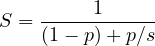
and it never exceeds  , however large is.
Proof. The original time, normalised to 1, splits into a part that is not sped up,  , and a sped-up part , which becomes
 . The new time is
 , and the speedup is the ratio of old to new time. As
 the denominator tends to . ∎
Examples.
- Speeding up by 4 times a part taking 80% of the time:
 . Even with infinite speedup it cannot exceed
 .
- A program that is 95% parallelisable on 16 cores:
 ; with infinitely many cores, at most 20.
The practical lesson: optimise the common case, and the part that stays slow always ends up dominating. Before optimising a program, measure where the time actually goes (with a profiler) instead of guessing.
The rest of the course
The next lessons follow the path of an instruction: how it is encoded (instruction set), how hardware does arithmetic, how the processor executes it (datapath and pipeline), where it finds the data (caches and virtual memory), how it talks to the outside world (input and output) and how several processors work together (parallelism).