Pipelining: stages, hazards, forwarding and branch prediction
The five stages, speedup with proof, data hazards and forwarding, load-use stall, control hazards and prediction, CPI with an example, superscalar processors.
In a laundry with a washer, a dryer and an iron, you do not wait for the first load to be ironed before putting the second in the washer: while the first dries, the second washes. Each load takes the same time, but one comes out every stage instead of every three. This is the idea of the pipeline: the datapath is split into stages, and each stage works on a different instruction. In this lesson we look at the classic five-stage pipeline, how much it gains and the hazards that slow it down.
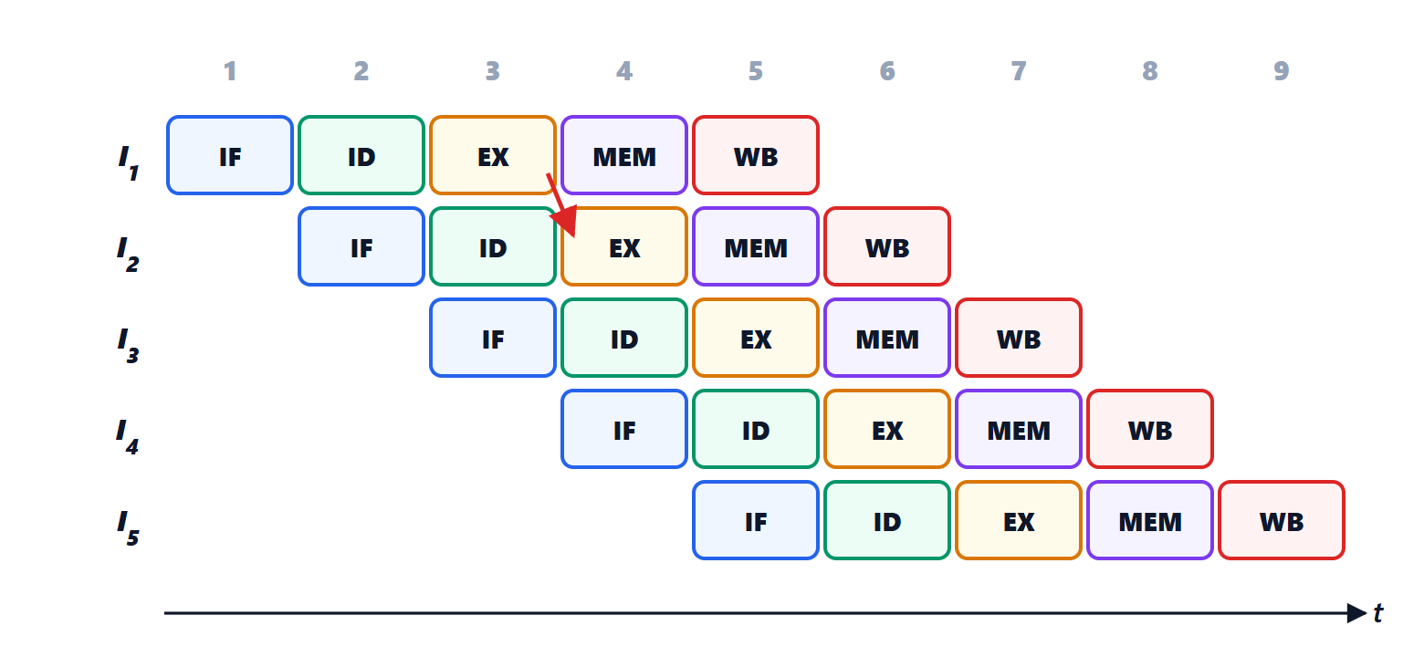
The five stages
- IF (fetch): reads the instruction and computes PC + 4;
- ID (decode): decodes and reads the registers;
- EX (execute): the ALU computes the result or the address;
- MEM (memory): reads or writes data memory;
- WB (write back): writes the result into the register file.
Between one stage and the next there are pipeline registers, which hold intermediate results and pass them to the next stage on the clock edge.
The gain
The clock period is now that of the slowest stage (about 200 ps in the example of the previous lesson, instead of 700).
Theorem. With  stages of equal duration,
 instructions take
 cycles, and the speedup over non-pipelined execution is
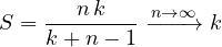
Proof. The first instruction comes out after cycles; from then on one comes out every cycle, so the other  take more cycles. Without a pipeline each instruction takes cycles of the same period, that is
 in total. ∎
With 5 stages and a million instructions the speedup is practically 5. The pipeline does not make a single instruction faster (it actually slows it slightly because of the extra registers), but it increases the number of instructions completed per unit time.
In practice the stages are not perfectly balanced and, above all, there are hazards, situations in which an instruction cannot proceed to the next cycle.
Data hazards
add  x5, x6, x7
sub  x8, x5, x9     # uses x5, which add has not written yet
add writes x5 in the WB stage, in the fifth cycle; sub reads it in the ID stage, in the third. Without countermeasures it would read the old value.
- Forwarding: the result is already available at the ALU output at the end of the third cycle; a multiplexer carries it directly to the ALU input for the next instruction, bypassing the register file. It solves most cases without losing cycles.
- Load followed by use: with
lw x5, 0(x6)followed by an instruction using x5, the data only arrives at the end of the MEM stage, too late for the next instruction’s EX. A one-cycle stall is needed (a “bubble” in the pipeline). The compiler often reorders instructions to fill that slot with an independent one.
Control hazards
A conditional branch is resolved only in the EX stage: meanwhile the pipeline has already fetched the following instructions, which may be the wrong ones. If the branch is taken they must be discarded, and two cycles are lost.
The solution is branch prediction: the processor guesses whether the branch will be taken and fetches accordingly; if it guesses wrong, it discards the work done. Modern predictors remember the past behaviour of each branch and guess right more than 95% of the time: a for loop always branches back, except on the last iteration.
Example. In a program 20% of instructions are loads, half of them immediately followed by a use (1 stall cycle); 15% are branches, mispredicted 10% of the time (2 cycles lost). The average CPI is

close to the ideal value of 1.
Beyond the simple pipeline
- Deeper pipelines: more, shorter stages allow higher frequencies, but raise the cost of mispredictions. Current processors have 10 to 20 stages.
- Superscalar: several pipelines in parallel, issuing two, four or more instructions per cycle (CPI below 1).
- Out-of-order execution: the processor looks ahead dozens of instructions and runs first those whose operands are ready, while the others wait for data from memory; results are then made visible in the original order.
All of this is invisible to the programmer: the program behaves as if instructions were executed one at a time, in the order written.