Branch prediction: two-bit counters, correlating predictors and targets

In a typical program one instruction in five or six is a branch. In a processor with a deep pipeline and a wide out-of-order window, every branch whose direction is unknown would block the flow for tens of cycles. The solution is to guess, and to do it very well: modern predictors miss fewer than one branch in a hundred. In this lesson we look at the cost of a misprediction, two-bit counters with the proof of their advantage on loops, correlating predictors, target prediction and how to write code that predictors like.

The cost of a misprediction

When the processor finds out it predicted wrongly, it discards all the speculative instructions and restarts from the right address (lesson on out-of-order execution). The cycles lost, the penalty, are about as many as it takes from instruction fetch to branch resolution: 15-20 in modern processors. With the performance equation with stalls:

with the fraction of instructions that are branches, the fraction mispredicted and the penalty. With 20 % branches, 5 % mispredictions and a 15-cycle penalty, 0.15 cycles per instruction are added: on a processor that could commit 4 per cycle (ideal CPI 0.25), execution time grows by 60 %. Every percentage point of accuracy counts.

Static prediction and one-bit counters

Static prediction decides without looking at history: for instance “backward branches are taken” (they are almost always loop closures) and “forward ones are not”. It works for about 70 % of branches.

The simplest dynamic prediction remembers, for each branch, what it did last time: one bit, in a table indexed by some bits of the branch address. It has an obvious flaw on loops.

The two-bit counter

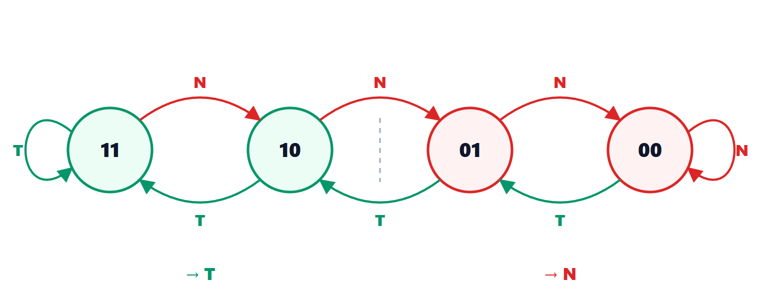
The two-bit saturating counter counts from 0 to 3: it increases when the branch is taken, decreases when it is not, without going past the ends. It predicts “taken” in states 2 and 3, “not taken” in states 0 and 1.

Theorem. An inner loop with iterations, executed repeatedly, has a closing branch taken times and not taken at the last. The one-bit predictor mispredicts twice per execution of the loop, the two-bit one only once.

Proof. *One bit.* At the last iteration the bit says “taken” (it was last time) and the branch is not: first misprediction, and the bit becomes “not taken”. At the first iteration of the next execution the bit says “not taken” but the branch is taken: second misprediction. The other iterations are predicted correctly. *Two bits.* After the taken iterations the counter is at 3. At the last iteration it predicts “taken” and is wrong, but it only drops to 2, which still predicts “taken”. At the first iteration of the next execution the prediction is right and the counter returns to 3. Only one misprediction per execution. ∎

With , accuracy goes from 80 to 90 %. The hysteresis of the counter prevents an isolated exception from changing the prediction.

Correlating predictors

Many branches depend on what earlier branches did: if an if (x > 0) was taken, a following if (x < 0) will not be. A correlating predictor keeps a global history register, the outcomes of the last branches executed (1 if taken, 0 if not), and uses it together with the branch address to choose the counter. In the gshare predictor the table index is the XOR of the address bits and the history bits: the same branch uses different counters in different contexts.

Today’s predictors, such as the TAGE family, combine tables with histories of different lengths, from a few branches to hundreds, and choose the prediction of the table with the longest history that has reliable information. They reach accuracies of 97-99 % on typical programs. Some also use small perceptrons, an elementary form of neural network.

Predicting where to jump too

Knowing that a branch is taken is not enough: one must know where it goes, even before the instruction has been decoded. The branch target buffer (BTB) is a cache indexed by the instruction address that returns last time’s destination address. Function returns have a dedicated predictor, the return address stack, which mimics the call stack: at every call the return address is pushed, at every return it is popped. Indirect branches (calls to virtual functions, switch statements compiled into tables) have predictors that also use history.

Writing predictable code

The predictor works no miracles with branches that depend on random data. The classic example: a loop that adds only the array elements greater than a threshold runs much faster if the array is sorted, because the branch becomes a long run of “not taken” followed by a long run of “taken”. On random data the predictor is wrong half the time. The countermeasures:

• turn the branch into a branch-free operation, with conditional moves (cmov on x86, select in RISC-V with extensions) or with arithmetic: sum += (x > threshold) * x. Compilers do it by themselves when both branches are short;
• reorder the data or the tests, putting the most frequent cases first;
• with execution profiles, let the compiler lay out the code so that the common path does not branch.