SIMD, GPUs and the roofline model
Processor vector extensions, the GPU SIMT model, divergence and coalesced accesses, arithmetic intensity, the roofline model with proof, the examples of the dot product and the matrix product.
Many programs spend almost all their time repeating the same operation on large amounts of data: filtering images, multiplying matrices, training neural networks, simulating physics. For this kind of work a different architecture pays off: a single instruction acting on many data at once. In this lesson we look at the SIMD vector extensions of processors, the GPU execution model with its constraints, and the roofline model, which with a two-line proof says whether a program is limited by computation or by memory.
SIMD in processors
In Flynn’s classification, SIMD (single instruction, multiple data) denotes a single instruction applied to several data. Modern processors have vector registers 128, 256 or 512 bits wide: a 256-bit register holds eight 32-bit floating-point numbers, and a single instruction adds them pairwise to those of another register. The main families are SSE and AVX on x86, NEON and SVE on ARM, the V extension on RISC-V.
SVE and RISC-V V are vector-length agnostic: the program asks the processor how many elements it can handle at a time and adapts, so the same code runs on processors with registers of different lengths. Compilers automatically vectorise simple loops, provided there are no dependences between iterations and the data are contiguous in memory.
The GPU model
A GPU pushes the idea to the extreme. It contains tens of streaming multiprocessors (SMs), each with tens of simple compute units, thousands in all. The programmer writes a function (the kernel) for a single element and launches it over millions of elements; the hardware groups threads in sets of 32 (warps) that execute the same instruction at the same time, each on its own data. This is the SIMT model (single instruction, multiple threads).
Two rules decide performance:
- divergence: if within a warp some threads take one branch of an
ifand others the other, the two branches are executed one after the other, with half the threads idle. GPU code must avoid branches that depend on the data of the single element; - coalesced accesses: if the 32 threads of a warp read 32 consecutive addresses, memory serves them with a single wide transfer; if they read scattered addresses, 32 transfers are needed.
GPUs do not hide memory latency with huge caches and out-of-order execution, but with numbers: each SM keeps tens of warps alive and, when one waits for memory, switches to another in one cycle. A great deal of parallelism is therefore needed, tens of thousands of active threads.
The roofline model
How fast can a program run on a given machine? Two limits matter: the peak compute performance  (operations per second) and the memory bandwidth
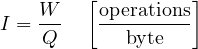
 (bytes per second). The link between the two is given by the program’s arithmetic intensity, the ratio of operations performed to bytes transferred from memory:
Theorem (roofline). The attainable performance is bounded by

Proof. The program performs  operations and transfers
 bytes in a time
 . The operations cannot be executed faster than the peak, so
 ; the bytes cannot be transferred faster than the bandwidth, so
 . Performance is
 , and from the two inequalities
 and
 . ∎
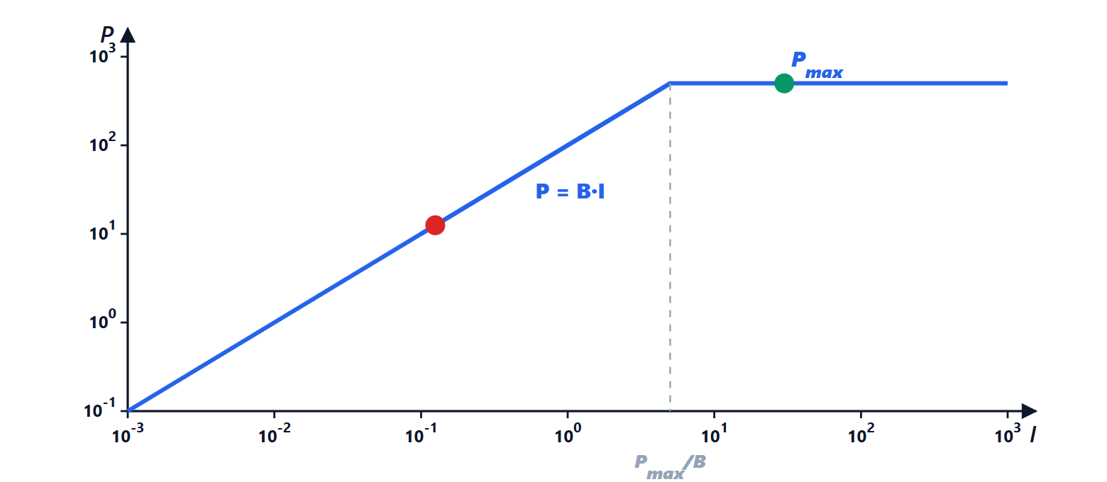
On a logarithmic scale the plot has the shape of a roof: a slope on the left and a flat top on the right, meeting at the ridge point  . A program with intensity below
 is memory-bound: improving computation is useless, transfers must be reduced. One with higher intensity is compute-bound.
Examples. A machine with  GFLOP/s and
 GB/s has its ridge at 5 operations per byte.
- The dot product of two 64-bit vectors performs 2 operations (a multiplication and an addition) every 16 bytes read:
 . Performance cannot exceed
 GFLOP/s, 2.5 % of the peak, however optimised the code.
- The matrix product with blocking (lesson on caches) performs
 operations while transferring about
 numbers: the intensity grows with the block side
 , and with large enough blocks the program becomes compute-bound. That is why matrix multiplication is the operation on which GPUs and AI accelerators reach their advertised performance.
The model extends to several roofs (with and without vector units, with data in cache or in DRAM) and guides optimisation: first measure where the program lies, then decide whether to work on data locality or on computation.