Instruction-level parallelism: dependences and register renaming
True, anti and output dependences, register renaming with proof, the performance equation with stalls, loop unrolling, the limits of ILP.
The Computer Systems course showed the five-stage pipeline, which overlaps the execution of successive instructions. But a simple pipeline reaches at most one instruction per cycle, and stops every time an instruction waits for the result of another. To go further one must understand which instructions can really be executed together. In this lesson we classify dependences, prove that only true ones limit parallelism while the others are removed by renaming registers, write the performance equation with stalls and look at loop unrolling.
Instruction-level parallelism
Instruction-level parallelism (ILP) is the possibility of executing several instructions of the same sequential program at the same time. The programmer writes a sequence; the processor must guarantee that the result is the same as executing it one instruction at a time, but it is free to change the order and to overlap everything that does not change the result.
Dependences
Between two instructions,  preceding
 in the program, there are three types of register dependence:
- true or data dependence (RAW, read after write): reads a register written by . The value must pass from one to the other: cannot compute before has produced its result;
- anti-dependence (WAR, write after read): writes a register that reads. If wrote first, would read the wrong value;
- output dependence (WAW, write after write): both write the same register. In the end the value of must remain.
To these are added control dependences, on conditional branches, and dependences through memory, harder to see because addresses are known only during execution.
True dependences and name dependences
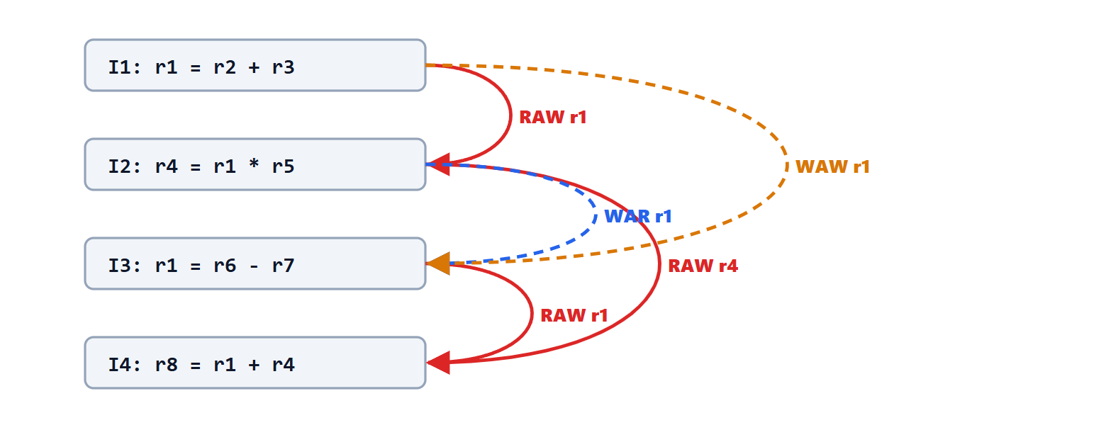
Anti-dependences and output dependences carry no data: they exist only because two different values use the same register name. In the example in the figure,  reuses
 for a value that has nothing to do with that of
 .
Theorem. If every instruction writes its result to a new physical register, never used before, and every read refers to the physical register of the last preceding write in the program, WAR and WAW dependences disappear and only RAW ones remain.
Proof. A WAW requires two writes to the same register: with a new physical register for every write there are none. A WAR requires to write a register that reads; but reads the physical register of the write preceding , while writes a new register, different from all existing ones, hence different from the one read. Finally, every read finds the value of the write that precedes it in the program, i.e. the same value as in sequential execution: the result does not change. ∎
This is register renaming. The processor has many more physical registers (hundreds) than the architectural ones visible to the programmer (32 in RISC-V), and a register alias table (RAT) that says, for every architectural register, which physical register holds the most recent value. In the example, after renaming, and are independent and can be executed together: only the red arrows remain.
The performance equation with stalls
Execution time is  (lesson on von Neumann and performance). In a pipeline the ideal CPI is 1, and every stall increases it:

where  is the frequency (per instruction) of a certain type of hazard and
 the number of cycles lost each time. For example, if 25 % of instructions are loads from memory and half of them are immediately followed by an instruction using the data, with one cycle lost each time, the contribution is
 : the CPI goes from 1 to 1.125, and the processor is 12.5 % slower.
Loop unrolling
The compiler can increase the available ILP. Consider a loop that adds a constant to every element of an array: each iteration loads, adds, stores, increments the index and branches. The three useful instructions depend on one another, and empty cycles remain in between, waiting for results.
By unrolling the loop four times, i.e. writing four iterations in the body with different registers, four independent chains are obtained. The compiler interleaves them: while the first addition waits for its load, the loads of the other three are executed. The empty cycles disappear, and the index increment and the branch, executed once every four elements instead of at every element, weigh a quarter as much. The price is longer code and more registers in use. Compilers do it automatically with optimisation options, and the same idea underlies vectorisation (lesson on SIMD and GPUs).
How much ILP is there really
Studies of ideal processors, with infinite units and perfect prediction, find tens of instructions executable in parallel in common programs. Real processors, limited by prediction, windows and memory, exploit 2 to 5 per cycle. The next lessons show the techniques that approach this: out-of-order execution, branch prediction, superscalar processors.