Solved digital control exercises: stability, discrete locus, delay and sampling
Eight exercises with solutions and graphs: Jury at third order, first-order process and deadbeat, integrator with delay, bilinear and Routh, sampled motor, computation delay, choice of sampling period, continuous versus discrete.
Exercises on the stability and design of digital control systems of the kind set in Digital Control courses, in three levels: basic, with the Jury criterion and the maximum gains of simple systems; intermediate, with the discrete root locus and the bilinear transformation; exam, with computation delay, the choice of the sampling period and the comparison between continuous and discrete. The result is given straight away; the full solution, with the graph, opens with a click. The proofs and the MATLAB and Python code are in the in-depth study linked at the top.
Basic level
Exercise 1. Jury at third order
Determine whether  has all its roots inside the unit circle, without computing them.
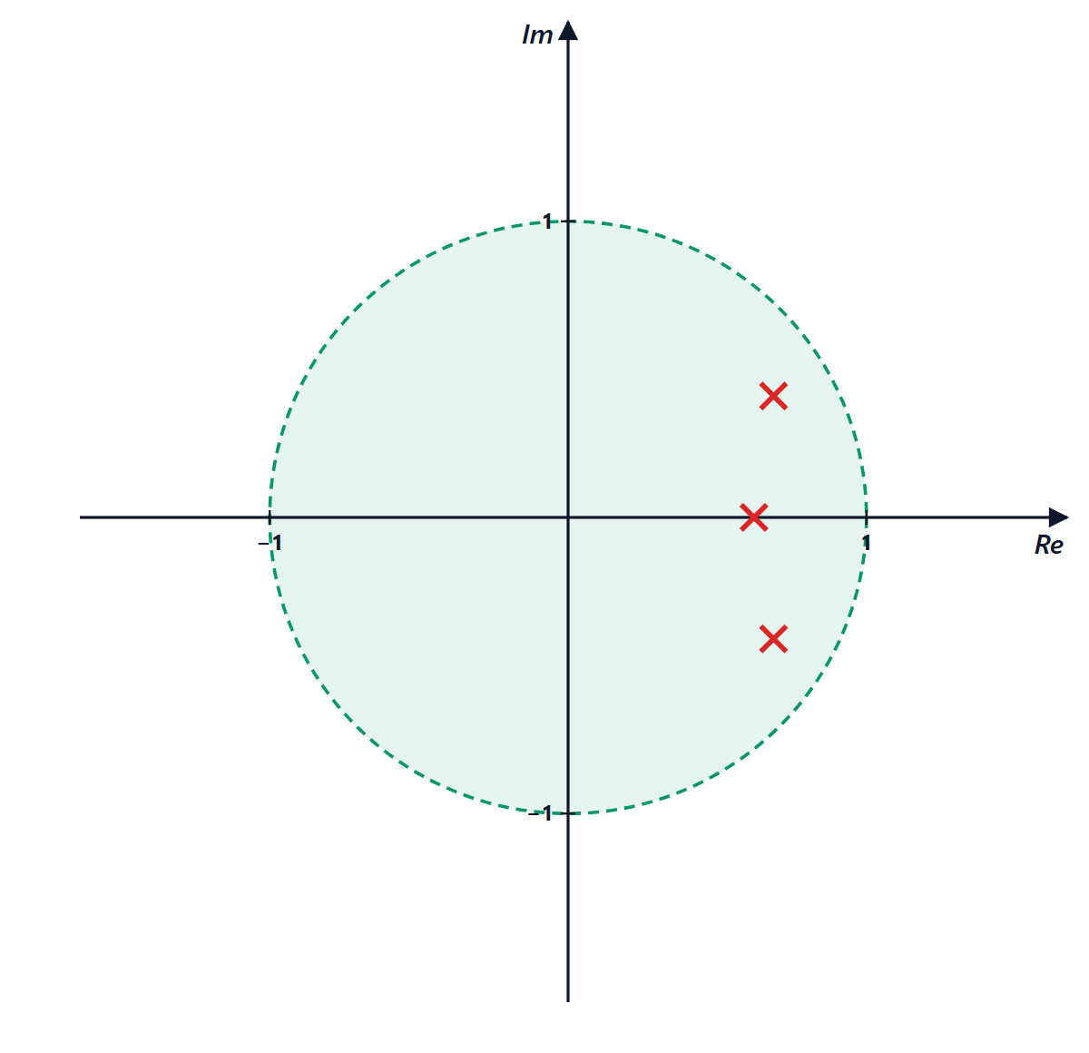
Result: yes: all the Jury conditions are satisfied (the roots have moduli 0.80, 0.80 and 0.62).
Solution
Coefficients:  ,
 ,
 ,
 .
1.  .
2.  .
3.  .
4.  .
Stable. The margin is small ( and condition 4 only just holds): the roots, computed afterwards, are
 and
 , with maximum modulus 0.80.
Exercise 2. A first-order process
The process  is controlled by a digital proportional controller with
 s and hold. Find the maximum gain, the steady-state step error with
 and the gain that puts the pole at
 .
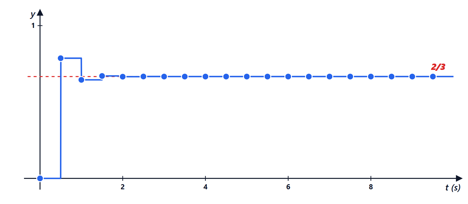
Result:  ; error
 ;
 .
Solution
ZOH:  . Closed loop:
 , pole
 .
Stability:  requires
 , i.e.
 . In continuous time, for the same process, there is no limit.
Steady-state error:  , so
 with : the output goes to
 . Without an integrator the error remains.
Pole at zero:  . The output reaches steady state in a single step (deadbeat response): a behaviour impossible in continuous time.
With the pole is  , negative: the response oscillates slightly from sample to sample.
Exercise 3. The period sets the gain
An integrator  is controlled with a gain
 ; the controller applies the command with one step of computation delay. With
 ms, what is the maximum gain? And the gain at which the poles break away?
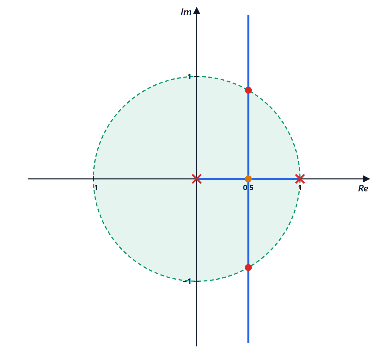
Result:  s
 ; breakaway for
 s.
Solution
From the lesson, with the delay the polynomial is  and Jury gives
 . With
 : .
The breakaway is halfway between the poles 0 and 1, where the polynomial has a double root: discriminant  ,
 , . For
 the response does not oscillate; between 25 and 100 it oscillates more and more; at the limit it has 6 samples per period.
To get more gain without losing stability one must sample faster:  is inversely proportional to
 .
Intermediate level
Exercise 4. Bilinear transformation and Routh
For which  is the system with characteristic polynomial
 stable? Use the bilinear transformation and check with the root locus.
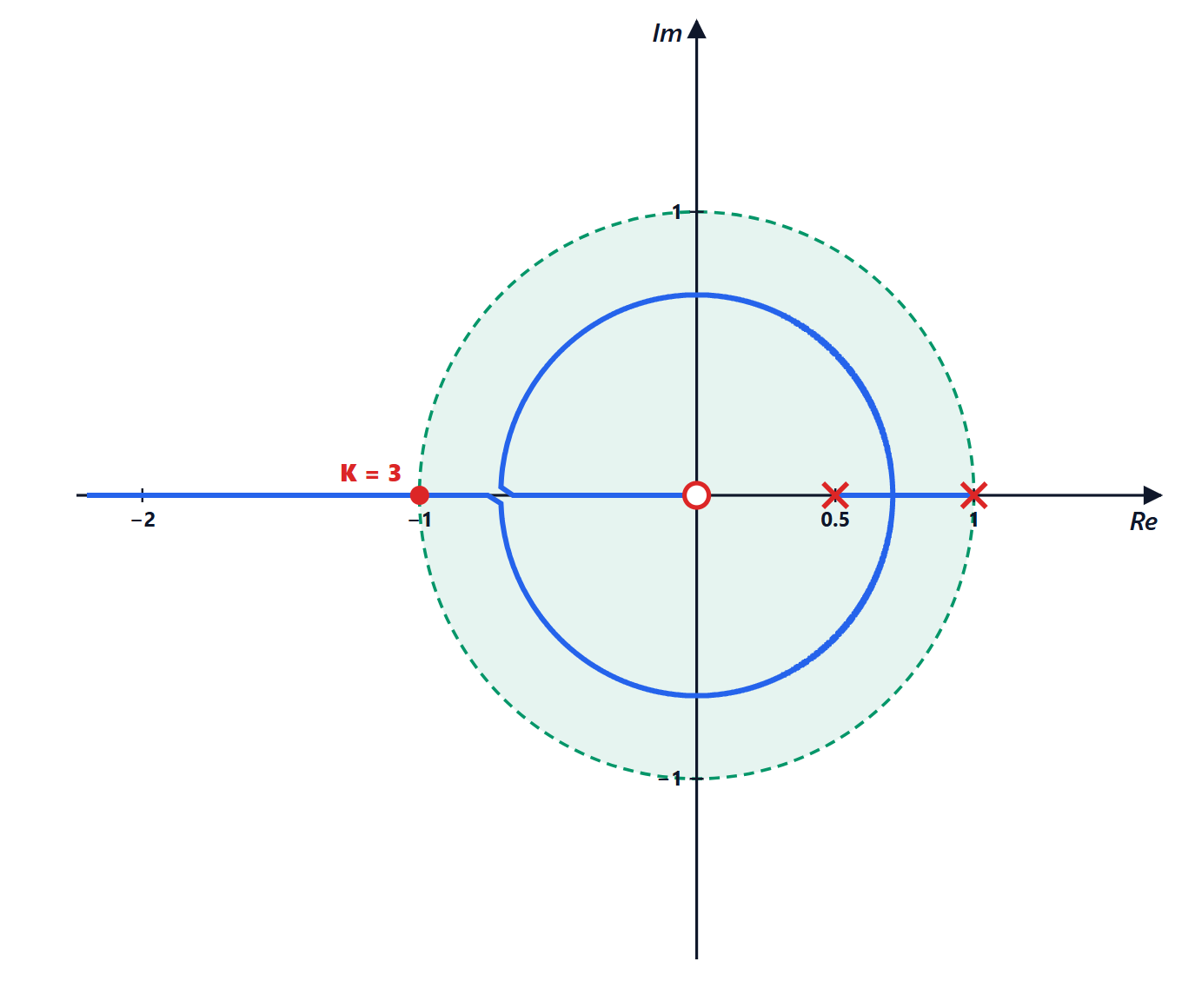
Result:  .
Solution
With  and
 , the transformed polynomial (in-depth study) is

Routh for second order: all coefficients positive, .
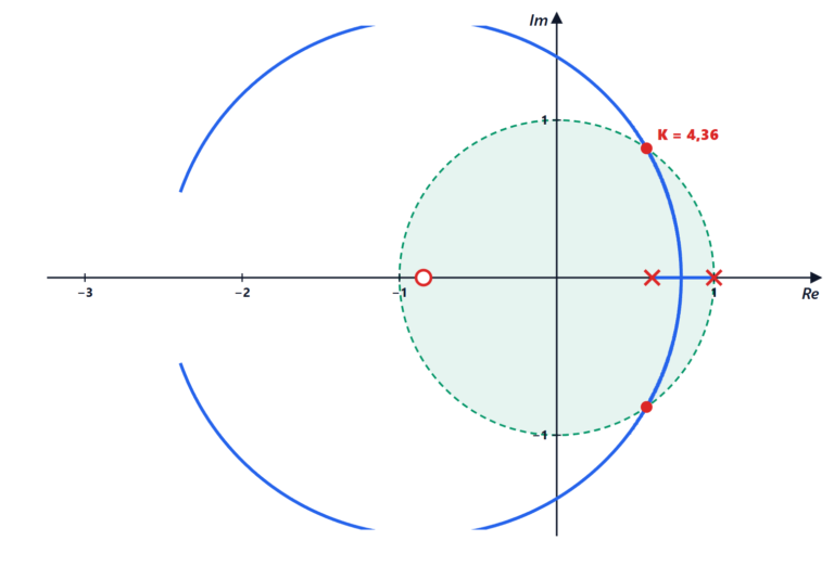
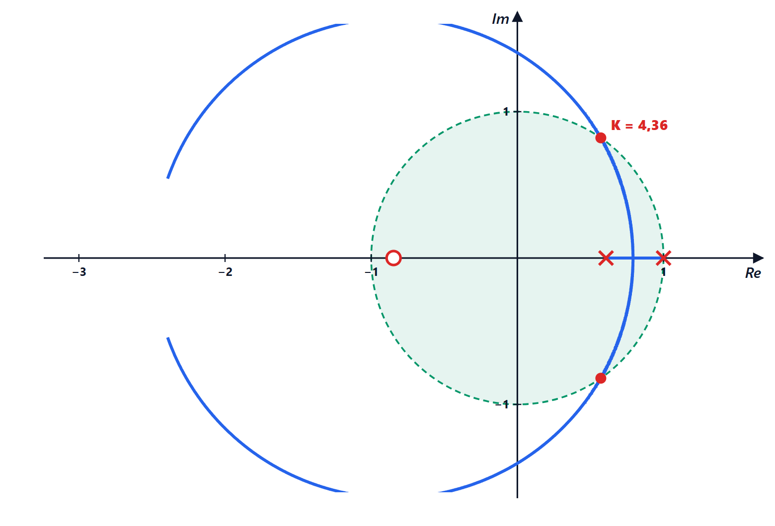
Locus. The polynomial is  : the locus of
 , with poles at 1 and 0.5 and a zero at 0. It is a circle centred at the zero with radius
 (continuous locus lesson: same geometry). The poles leave the unit circle on the real axis, at
 , when
 .
Exercise 5. The sampled motor
For the motor  sampled with s (in-depth study), check
 with Jury and find the frequency of the oscillation at the limit.
Result: ; oscillation with period 3.3 s (6.5 samples).
Solution
Polynomial  . The binding Jury condition is
 :
 ,
 (the others give and
 ).
For  :
 ,
 , angle
 rad. The angular frequency of the oscillation is
 rad/s, the period
 s, i.e. 6.5 samples.
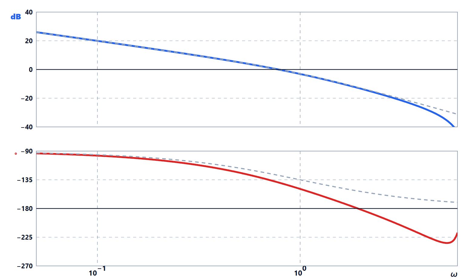
It is the same frequency  rad/s at which the phase of the discrete Bode plot is
 : Jury, locus and Nyquist give the same information.
Exam level
Exercise 6. The price of computation delay
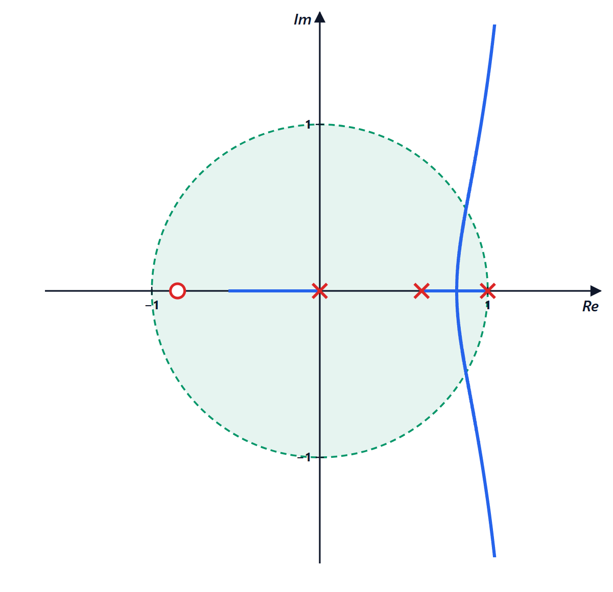
One step of computation delay is added to the sampled motor of exercise 5: 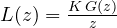 . How do the maximum gain and the phase margin with
 change?
Result: falls from 4.36 to 1.49; the phase margin from 40.8° to 18.3°.
Solution
The characteristic polynomial becomes third order:  . With Jury, or by computing the roots as varies (code of the in-depth study with
 ), one finds
 .
In frequency,  has magnitude 1 and phase
 : at the crossover frequency (about 0.78 rad/s) it removes
 rad, i.e. 22.4°. The margin falls from 40.8° to 18.3°.
Remedies: sample faster (the delay, in seconds, gets shorter), or apply the command as soon as it is computed instead of at the next step, keeping the code between the A/D read and the D/A write to a minimum (lesson on implementation).
Exercise 7. Choosing the sampling period
A continuous control loop has crossover frequency  rad/s and a phase margin of 60°. Which sampling period guarantees losing no more than 5° of margin because of the hold? And if there is also one step of computation delay?
Result:  ms; with the computation delay
 ms.
Solution
The hold is equivalent to a delay of  : phase loss
 . Requiring
 rad:
 ms.
With one more step of delay the total delay is  :
 ms.
Equivalent rule of thumb: sample 20-40 times faster than the loop bandwidth ( Hz, so at least 30-60 Hz; at 170 Hz one is well on the safe side). In car ECUs fast controllers run at 1-10 ms, slow ones (temperature, level) at 100 ms.
Exercise 8. Continuous versus discrete with the same gain
The motor  is controlled with : compare the overshoot of the continuous system and of the one sampled with s. Write the commands to check it.
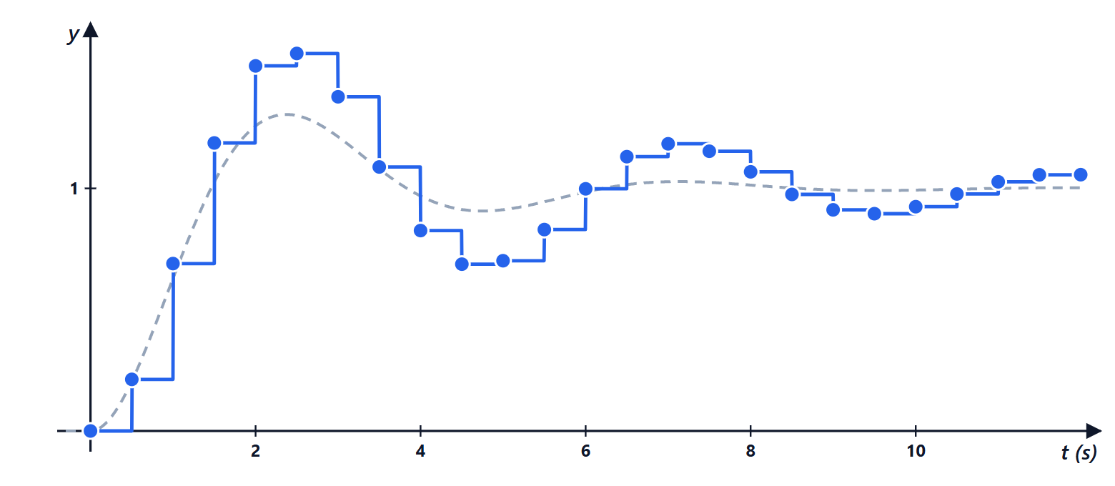
Result: continuous 30.5 %; sampled 55.6 %.
Solution
Continuous:  ,
 ,
 , overshoot
 %.
Sampled: polynomial  , roots
 , modulus 0.887, angle 38.2°. The equivalent continuous pole
 has
 : much less damped, overshoot about 56 %.
MATLAB: G = tf(1,[1 1 0]); stepinfo(feedback(2*G,1)), stepinfo(feedback(2*c2d(G,0.5),1)). Python: ct.step_info(ct.feedback(2*G, 1)) and ct.step_info(ct.feedback(2*ct.sample_system(G, 0.5), 1)), which give 30.5 % and 55.6 %.
The lesson is general: a controller tuned in continuous time and placed in a slow processor loses damping. Either sample faster, or design directly in discrete time.