Microstrip antennas: the cavity model and patch design
Structure of the patch, the cavity model and the resonance condition proved, design formulas with a 2.45 GHz example, feeding and matching, bandwidth, circular polarisation, phone antennas.
The antennas of phones, GPS receivers, Wi-Fi routers and car radars are neither wires nor dishes: they are copper rectangles printed on a circuit board, microstrip antennas (patches). They are flat, light, cheap, integrate with the electronics and are easily put into arrays. In this lesson we look at how a patch is made, the resonance condition derived with the cavity model, the design formulas with a complete numerical example, matching, bandwidth and circular polarisation, and phone antennas.
The structure
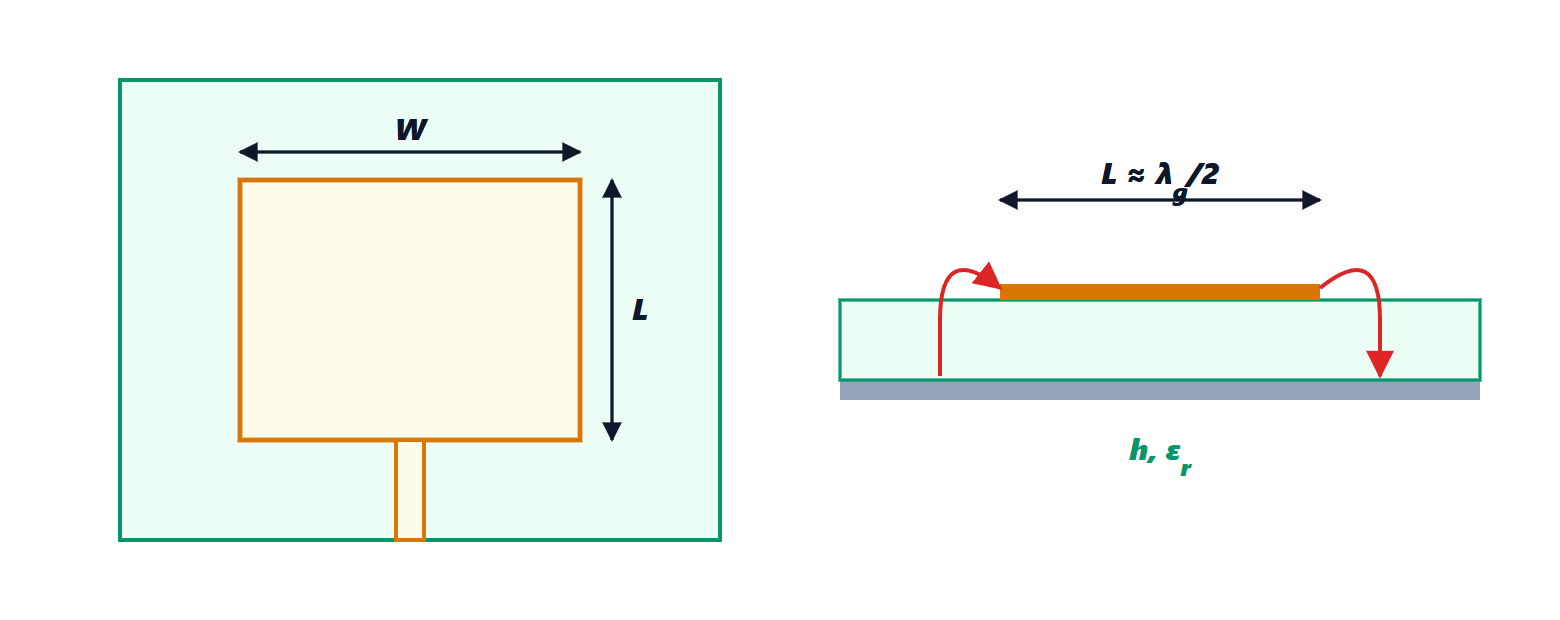
A patch is a rectangular metal sheet, of length  and width
 , on a dielectric substrate of thickness
 and relative permittivity
 , with a ground plane underneath. It is fed by a microstrip line printed on the same layer or by a coaxial probe through the substrate.
The cavity model
The space between the patch and the ground plane behaves like a resonant cavity. On the upper and lower metal surfaces the tangential electric field is zero, so the field is vertical, and since is small it does not vary through the thickness. On the four open edges the current on the patch must vanish, which amounts to saying that the magnetic field tangent to the edges is about zero: the edges behave as magnetic walls.
Theorem. The fundamental mode of a patch (TM₀₁₀) resonates when the effective length equals half a wavelength in the dielectric:
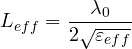
Proof. With magnetic walls at the two edges  and
 , the vertical electric field must have zero normal derivative on both, i.e. a maximum or a minimum: the simplest non-constant solution is
 , which has maxima of opposite sign at the two edges. The wavenumber along
 is
 , and at resonance it must equal the wavenumber in the medium,
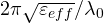 . Equating gives the formula. ∎
At the two edges the vertical field has opposite direction; the fringing fields leaving the substrate instead have horizontal components in the same direction (as seen in the cross-section of the figure): the two edges behave like two radiating slots in phase, half a wavelength apart, and the patch radiates mainly upwards, with a typical gain of 5-8 dBi.
Design formulas
The fringing field makes the patch look slightly longer than it is, by  on each side, and part of the field is in air: an empirical effective permittivity and extension are used. The classic formulas, for design frequency
 :


Example. A patch for 2.45 GHz Wi-Fi on FR4 glass-epoxy ( ,
 mm). The width comes out as
 mm. With
 , the effective permittivity is
 . Half a wavelength in the medium is
 mm, the extension
 mm, and the physical length
 mm. In practice the structure is simulated with an electromagnetic solver and is trimmed after the first measurement, because the permittivity of FR4 varies from batch to batch.
Matching and bandwidth
At the edge of the patch the input resistance is high, 200-300 Ω, because there the voltage is maximum and the current minimum. Moving the feed point towards the centre the resistance falls as  : with an inset feed (a notch in the patch that brings the microstrip line inwards) or with a probe at the right point, 50 Ω is obtained.
The patch is a cavity with few paths for energy to escape: it has a high quality factor and a narrow bandwidth, typically 1-5 %, which grows with substrate thickness and decreases with its permittivity. To widen it, thick low-permittivity substrates are used (even foam or air), stacked patches or U-shaped slots.
Circular polarisation
A square patch has two equal modes, along the two sides, at 90° to each other. Exciting them with equal amplitude and 90° out of phase gives circular polarisation, that of GPS satellites (lesson on parameters). A single feed is enough if two opposite corners of the square are cut off: the two modes acquire slightly different resonant frequencies, and at the frequency in between one leads and the other lags by 45°.
Phone antennas
In a phone space is minimal and the bands are many, from 600 MHz to 6 GHz. Variants of the patch are used such as the planar inverted-F antenna (PIFA), a quarter-wave patch shorted to ground on one side, and more and more often the phone’s own metal frame, divided into segments and tuned with switches. The user’s body, holding the phone in hand or next to the head, changes the matching and absorbs power: modern phones continuously measure the load and retune the antennas. At the millimetre waves of 5G (26-40 GHz) the wavelength is a few millimetres, and small patch arrays with beamforming are integrated directly into the radio module (lesson on arrays).