Antenna arrays: array factor, steering and grating lobes
Pattern multiplication, the array factor of the uniform linear array with proof, electronic steering, the condition against grating lobes proved, beamwidth, tapering, digital arrays and massive MIMO.
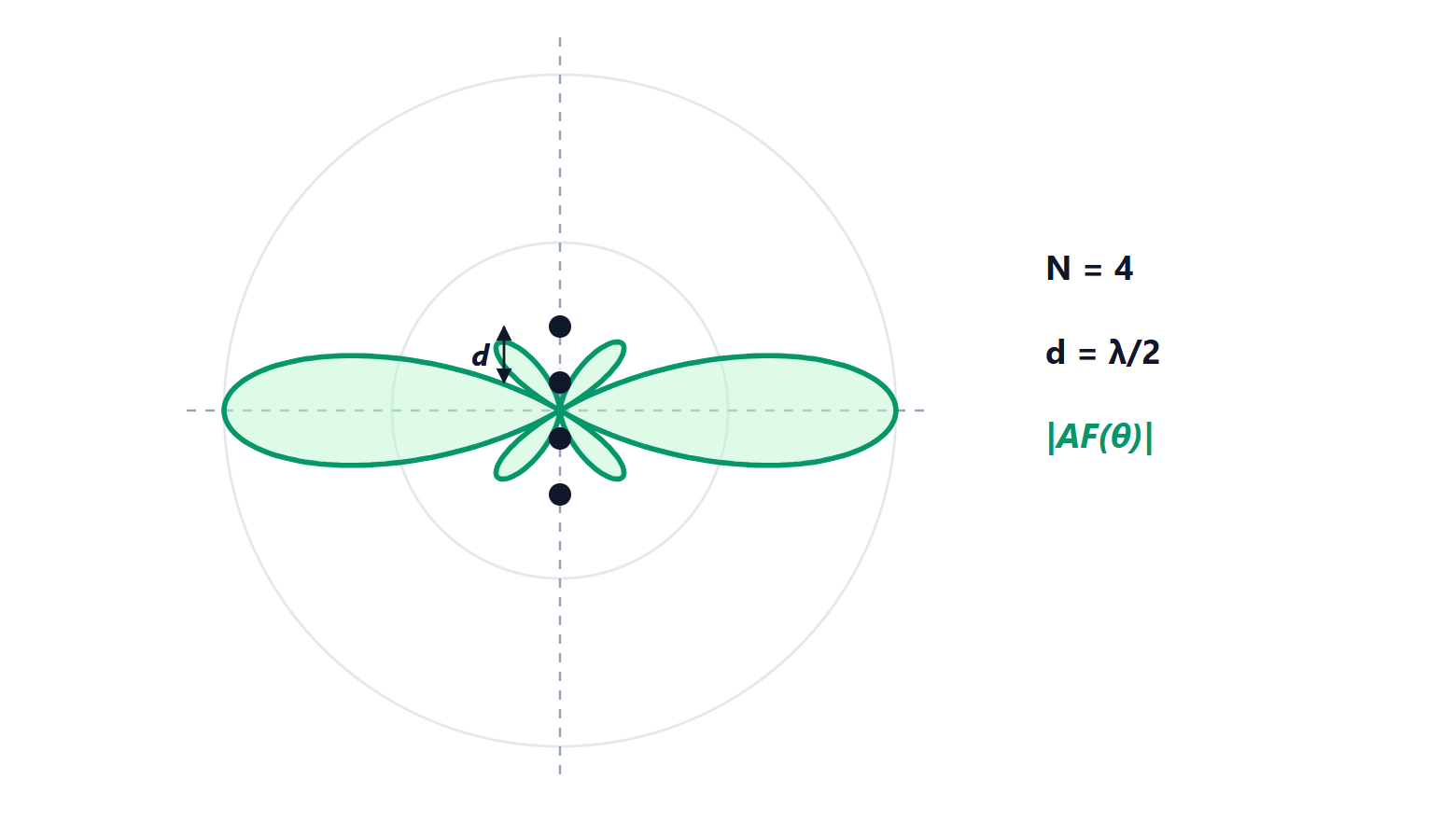
Putting together several identical antennas and feeding them with chosen amplitudes and phases gives a more directive antenna whose beam can be steered electronically, without moving anything. Phased arrays are in military and weather radars, in 5G base stations, in terminals for low-orbit satellites. The Electromagnetic Fields course introduced them. In this lesson we prove the array factor of a uniform linear array, see how the beam is steered, prove the condition for avoiding grating lobes, and look at beamwidth, side-lobe tapering and digital arrays.
The principle of pattern multiplication
An array of  identical, identically oriented elements has a field equal to the field of a single element multiplied by the array factor (AF), which depends only on the positions, amplitudes and feed phases:

The reason is that every element produces the same field, shifted in space: in the far field the shift becomes just a phase factor  (lesson on the far field).
The uniform linear array
Consider elements aligned along the  axis, with spacing
 , equal amplitudes and a phase increasing by
 from one element to the next. The total phase difference between adjacent elements, in direction
 , is

Theorem. The normalised array factor is
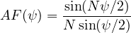
Proof.  , a geometric series with ratio
 , equal to
 . Factoring
 out of the numerator and
 out of the denominator leaves
 and
 , plus a phase factor of unit magnitude. ∎
It is the same function as the moving average (Digital Signal Processing lesson on the DTFT): an antenna array is a spatial filter, and angle plays the role of frequency. The maximum, equal to 1, occurs at  ; the zeros at
 ; the first side lobe is at −13.3 dB.
Steering the beam
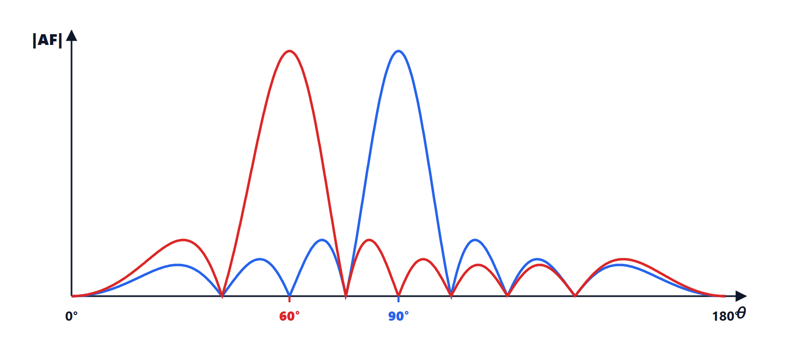
The maximum falls where , i.e.  . To point in direction
 it is therefore enough to choose

With  the beam is perpendicular to the array (broadside array); with
 it is along the array (endfire). Changing the phase shifters in a few microseconds moves the beam: this is electronic scanning.
Grating lobes
If the elements are too far apart, other lobes as high as the main one appear, the grating lobes, which scatter power in unwanted directions and confuse the direction of arrival.
Theorem. An array pointed in direction has no grating lobes in real space if
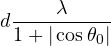
Proof.  equals 1 whenever
 is a multiple of
 . As goes from 0 to
 ,
 covers the interval
 , the visible region. With
 , the main lobe is at ; a grating lobe would appear if the visible region reached
 . Its end farthest from zero is
 in magnitude. It does not reach if
 , i.e.
 . ∎
For a broadside array  suffices; to be able to point all the way to the axis,
 is needed. That is why phased arrays almost always use half-wavelength spacing.
Beamwidth and side lobes
For a broadside array of length  , the half-power width is about
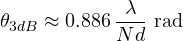
inversely proportional to the length in wavelengths. Pointing away from broadside the beam widens as  : the array “seen at an angle” looks shorter. With 8 elements at
 the beam is about 12.7° wide.
Side lobes at −13 dB are too high for a radar, which would see a strong target even outside the beam. The excitation is tapered: central elements receive more amplitude than edge ones, exactly like windows for FIR filters (lesson on windows). The Dolph-Chebyshev and Taylor distributions give side lobes at −30 or −40 dB, at the price of a slightly wider beam and a few tenths of a decibel of gain.
Planar and digital arrays
Placing the elements on a plane steers the beam in two dimensions. Modern arrays are active: each element has its own module with amplifiers and phase shifters, and a failure switches off only one of them. In digital arrays each element, or each small group, has its own converter, and beam formation (beamforming) takes place in the computer: many beams can be formed at once, towards different users. It is the principle of the massive MIMO of 5G base stations, with 64 or more elements, and of terminals for low-orbit satellites, which track a satellite crossing the sky in a few minutes with no moving parts.